Is There a Quantum Trajectory? The Phase-Space Perspective

At the dawn of quantum theory, Heisenberg, Schrödinger, Bohr and Pauli were embroiled in a dispute over whether trajectories of particles, defined by their positions over time, could exist. The argument against trajectories was based on an apparent paradox: To draw a “line” depicting a trajectory of a particle along a path implies that there is a momentum vector that carries the particle along that path. But a line is a one-dimensional curve through space, and since at any point in time the particle’s position is perfectly localized, then by Heisenberg’s uncertainty principle, it can have no definable momentum to carry it along.

My previous blog shows the way out of this paradox, by assembling wavepackets that are spread in both space and momentum, explicitly obeying the uncertainty principle. This is nothing new to anyone who has taken a quantum course. But the surprising thing is that in some potentials, like a harmonic potential, the wavepacket travels without broadening, just like classical particles on a trajectory. A dramatic demonstration of this can be seen in this YouTube video. But other potentials “break up” the wavepacket, especially potentials that display classical chaos. Because phase space is one of the best tools for studying classical chaos, especially Hamiltonian chaos, it can be enlisted to dig deeper into the question of the quantum trajectory—not just about the existence of a quantum trajectory, but why quantum systems retain a shadow of their classical counterparts.

Phase Space

Phase space is the state space of Hamiltonian systems. Concepts of phase space were first developed by Boltzmann as he worked on the problem of statistical mechanics. Phase space was later codified by Gibbs for statistical mechanics and by Poincare for orbital mechanics, and it was finally given its name by Paul and Tatiana Ehrenfest (a husband-wife team) in correspondence with the German physicist Paul Hertz (See Chapter 6, “The Tangled Tale of Phase Space”, in Galileo Unbound by D. D. Nolte (Oxford, 2018)).

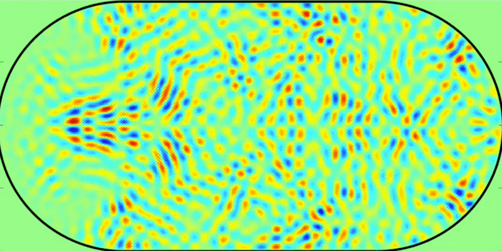
The stretched-out phase-space functions … are very similar to the stochastic layer that forms in separatrix chaos in classical systems.

The idea of phase space is very simple for classical systems: it is just a plot of the momentum of a particle as a function of its position. For a given initial condition, the trajectory of a particle through its natural configuration space (for instance our 3D world) is traced out as a path through phase space. Because there is one momentum variable per degree of freedom, then the dimensionality of phase space for a particle in 3D is 6D, which is difficult to visualize. But for a one-dimensional dynamical system, like a simple harmonic oscillator (SHO) oscillating in a line, the phase space is just two-dimensional, which is easy to see. The phase-space trajectories of an SHO are simply ellipses, and if the momentum axis is scaled appropriately, the trajectories are circles. The particle trajectory in phase space can be animated just like a trajectory through configuration space as the position and momentum change in time p(x(t)). For the SHO, the point follows the path of a circle going clockwise.

Fig. 1 Phase space of the simple harmonic oscillator. The “orbits” have constant energy.

A more interesting phase space is for the simple pendulum, shown in Fig. 2. There are two types of orbits: open and closed. The closed orbits near the origin are like those of a SHO. The open orbits are when the pendulum is spinning around. The dividing line between the open and closed orbits is called a separatrix. Where the separatrix intersects itself is a saddle point. This saddle point is the most important part of the phase space portrait: it is where chaos emerges when perturbations are added.

Fig. 2 Phase space for a simple pendulum. For small amplitudes the orbits are closed like those of a SHO. For large amplitudes the orbits become open as the pendulum spins about its axis. (Reproduced from Introduction to Modern Dynamics, 2nd Ed., pg. )

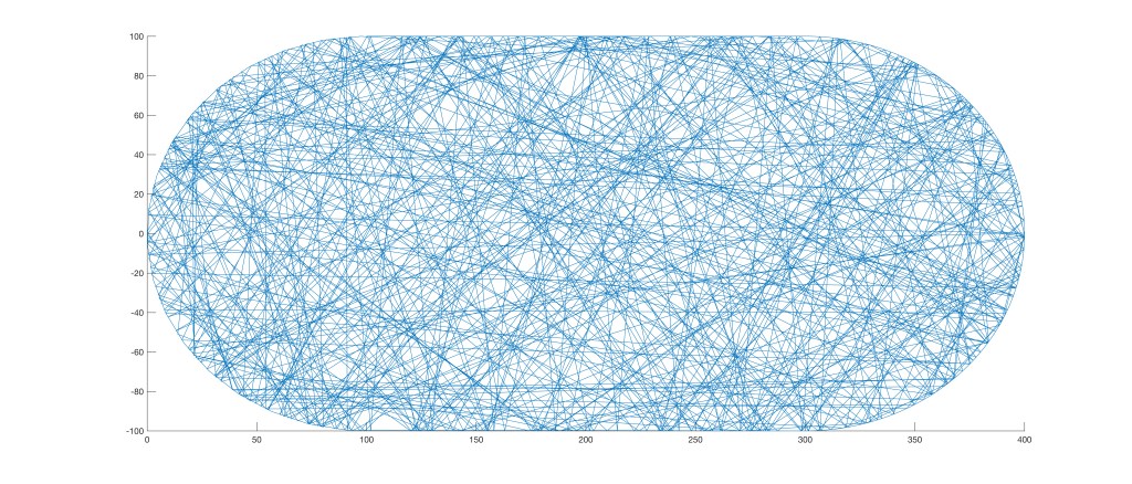
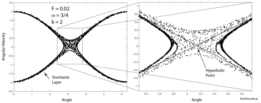
One route to classical chaos is through what is known as “separatrix chaos”. It is easy to see why saddle points (also known as hyperbolic points) are the source of chaos: as the system trajectory approaches the saddle, it has two options of which directions to go. Any additional degree of freedom in the system (like a harmonic drive) can make the system go one way on one approach, and the other way on another approach, mixing up the trajectories. An example of the stochastic layer of separatrix chaos is shown in Fig. 3 for a damped driven pendulum. The chaotic behavior that originates at the saddle point extends out along the entire separatrix.

Fig. 3 The stochastic layer of separatrix chaos for a damped driven pendulum. (Reproduced from Introduction to Modern Dynamics, 2nd Ed., pg. )

The main question about whether or not there is a quantum trajectory depends on how quantum packets behave as they approach a saddle point in phase space. Since packets are spread out, it would be reasonable to assume that parts of the packet will go one way, and parts of the packet will go another. But first, one has to ask: Is a phase-space description of quantum systems even possible?

Quantum Phase Space: The Wigner Distribution Function

Phase-space portraits are arguably the most powerful tool in the toolbox of classical dynamics, and one would like to retain its uses for quantum systems. However, there is that pesky paradox about quantum trajectories that cannot admit the existence of one-dimensional curves through such a phase space. Furthermore, there is no direct way of taking a wavefunction and simply “finding” its position or momentum to plot points on such a quantum phase space.

The answer was found in 1932 by Eugene Wigner (1902 – 1905), an Hungarian physicist working at Princeton. He realized that it was impossible to construct a quantum probability distribution in phase space that had positive values everywhere. This is a problem, because negative probabilities have no direct interpretation. But Wigner showed that if one relaxed the requirements a bit, so that expectation values computed over some distribution function (that had positive and negative values) gave correct answers that matched experiments, then this distribution function would “stand in” for an actual probability distribution.

The distribution function that Wigner found is called the Wigner distribution function. Given a wavefunction ψ(x), the Wigner distribution is defined as

Fig. 4 Wigner distribution function in (x, p) phase space.

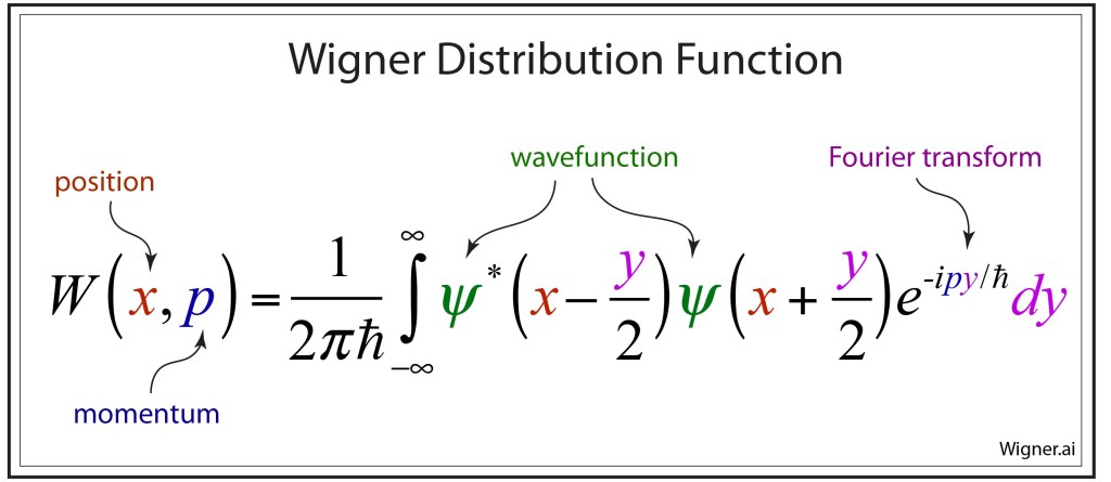
The Wigner distribution function is the Fourier transform of the convolution of the wavefunction. The pure position dependence of the wavefunction is converted into a spread-out position-momentum function in phase space. For a Gaussian wavefunction ψ(x) with a finite width in space, the W-function in phase space is a two-dimensional Gaussian with finite widths in both space and momentum. In fact, the Δx-Δp product of the W-function is precisely the uncertainty production of the Heisenberg uncertainty relation.

The question of the quantum trajectory from the phase-space perspective becomes whether a Wigner function behaves like a localized “packet” that evolves in phase space in a way analogous to a classical particle, and whether classical chaos is reflected in the behavior of quantum systems.

The Harmonic Oscillator

The quantum harmonic oscillator is a rare and special case among quantum potentials, because the energy spacings between all successive states are all the same. This makes it possible for a Gaussian wavefunction, which is a superposition of the eigenstates of the harmonic oscillator, to propagate through the potential without broadening. To see an example of this, watch the first example in this YouTube video for a Schrödinger cat state in a two-dimensional harmonic potential. For this very special potential, the Wigner distribution behaves just like a (broadened) particle on an orbit in phase space, executing nice circular orbits.

A comparison of the classical phase-space portrait versus the quantum phase-space portrait is shown in Fig. 5. Where the classical particle is a point on an orbit, the quantum particle is spread out, obeying the Δx-Δp Heisenberg product, but following the same orbit as the classical particle.

Fig. 5 Classical versus quantum phase-space portraits for a harmonic oscillator. For a classical particle, the trajectory is a point executing an orbit. For a quantum particle, the trajectory is a Wigner distribution that follows the same orbit as the classical particle.

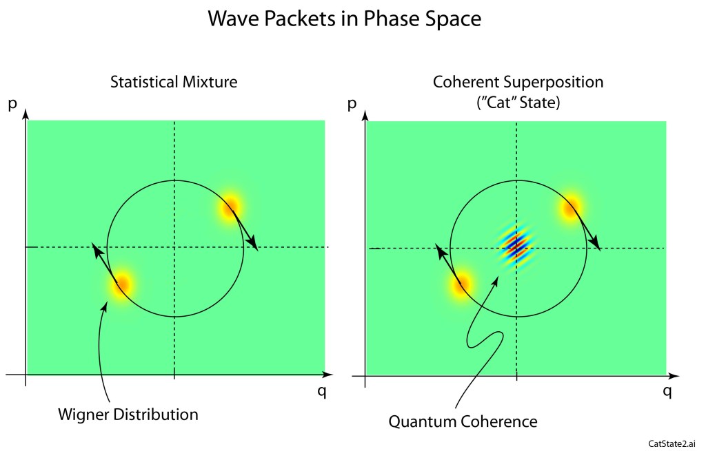
However, a significant new feature appears in the Wigner representation in phase space when there is a coherent superposition of two states, known as a “cat” state, after Schrödinger’s cat. This new feature has no classical analog. It is the coherent interference pattern that appears at the zero-point of the harmonic oscillator for the Schrödinger cat state. There is no such thing as “classical” coherence, so this feature is absent in classical phase space portraits.

Two examples of Wigner distributions are shown in Fig. 6 for a statistical (incoherent) mixture of packets and a coherent superposition of packets. The quantum coherence signature is present in the coherent case but not the statistical mixture case. The coherence in the Wigner distribution represents “off-diagonal” terms in the density matrix that leads to interference effects in quantum systems. Quantum computing algorithms depend critically on such coherences that tend to decay rapidly in real-world physical systems, known as decoherence, and it is possible to make statements about decoherence by watching the zero-point interference.

Fig. 6 Quantum phase-space portraits of double wave packets. On the left, the wave packets have no coherence, being a statistical mixture. On the right is the case for a coherent superposition, or “cat state” for two wave packets in a one-dimensional harmonic oscillator.

Whereas Gaussian wave packets in the quantum harmonic potential behave nearly like classical systems, and their phase-space portraits are almost identical to the classical phase-space view (except for the quantum coherence), most quantum potentials cause wave packets to disperse. And when saddle points are present in the classical case, then we are back to the question about how quantum packets behave as they approach a saddle point in phase space.

Quantum Pendulum and Separatrix Chaos

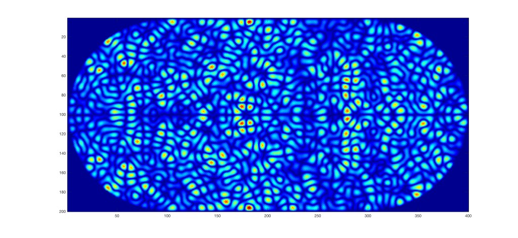
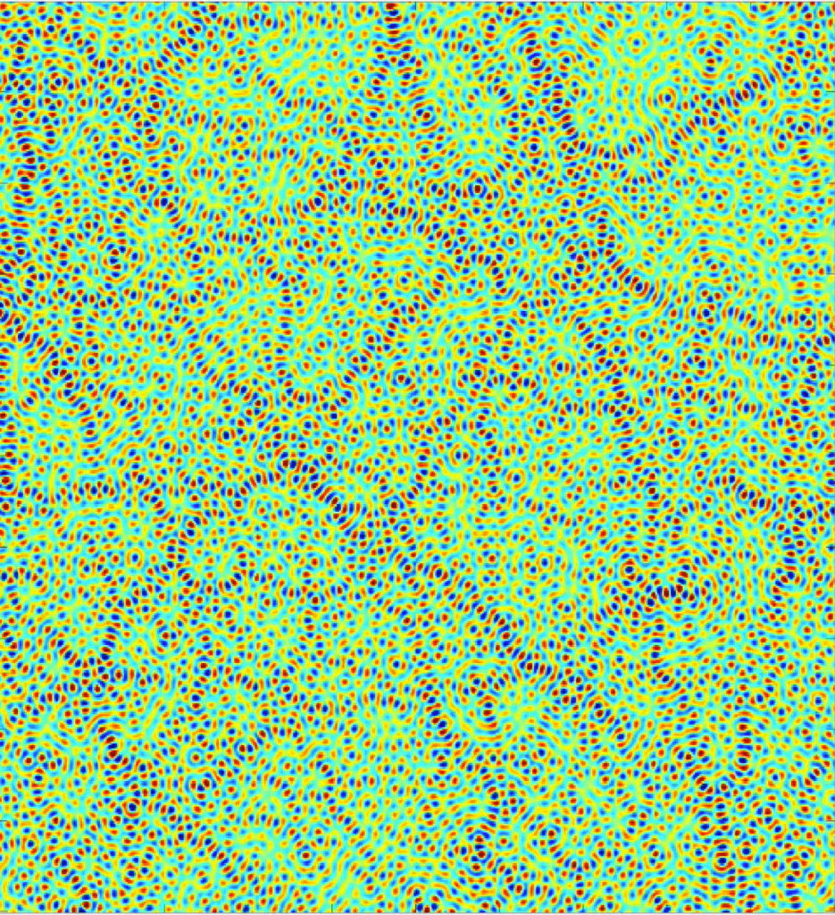
One of the simplest anharmonic oscillators is the simple pendulum. In the classical case, the period diverges if the pendulum gets very close to going vertical. A similar thing happens in the quantum case, but because the motion has strong anharmonicity, an initial wave packet tends to spread dramatically as parts of the wavefunction less vertical stretch away from the part of the wave function that is more nearly vertical. Fig. 7 is a snap-shot about a eighth of a period after the wave packet was launched. The packet has already stretched out along the separatrix. A double-cat-state was used, so there is a second packet that has coherent interference with the first. To see a movie of the time evolution of the wave packet and the orbit in quantum phase space, see the YouTube video.

Fig. 7 Wavefunction of a quantum pendulum released near vertical. The phase-space portrait is very similar to the classical case, except that the phase-space distribution is stretched out along the separatrix. The initial state for the phase-space portrait was a cat state.

The simple pendulum does have a saddle point, but it is degenerate because the angle is modulo -2-pi. A simple potential that has a non-degenerate saddle point is a double-well potential.

Quantum Double-Well and Separatrix Chaos

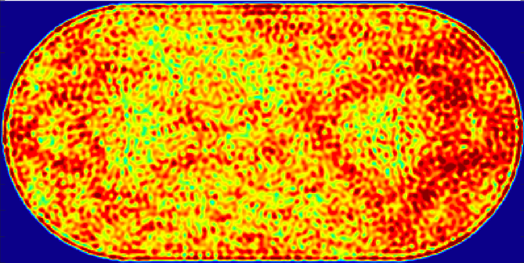
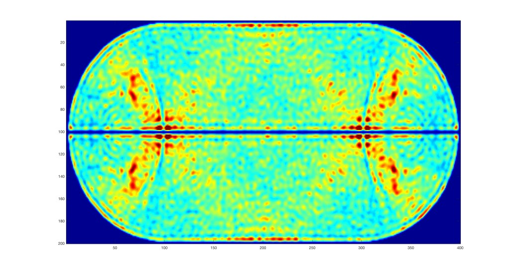
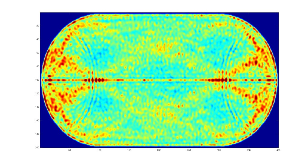
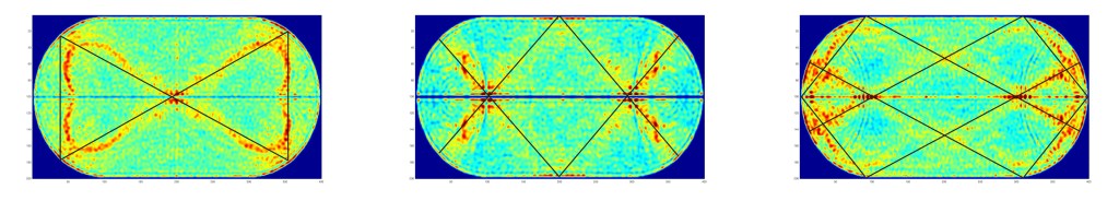
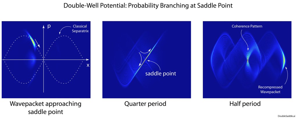
The symmetric double-well potential has a saddle point at the mid-point between the two well minima. A wave packet approaching the saddle will split into to packets that will follow the individual separatrixes that emerge from the saddle point (the unstable manifolds). This effect is seen most dramatically in the middle pane of Fig. 8. For the full video of the quantum phase-space evolution, see this YouTube video. The stretched-out distribution in phase space is highly analogous to the separatrix chaos seen for the classical system.

Fig. 8 Phase-space portraits of the Wigner distribution for a wavepacket in a double-well potential. The packet approaches the central saddle point, where the probability density splits along the unstable manifolds.

Conclusion

A common statement often made about quantum chaos is that quantum systems tend to suppress chaos, only exhibiting chaos for special types of orbits that produce quantum scars. However, from the phase-space perspective, the opposite may be true. The stretched-out Wigner distribution functions, for critical wave packets that interact with a saddle point, are very similar to the stochastic layer that forms in separatrix chaos in classical systems. In this sense, the phase-space description brings out the similarity between classical chaos and quantum chaos.

By David D. Nolte Sept. 25, 2022


YouTube Video

YouTube Video of Dynamics in Quantum Phase Space


References

1. T. Curtright, D. Fairlie, C. Zachos, A Concise Treatise on Quantum Mechanics in Phase Space.  (World Scientific, New Jersey, 2014).

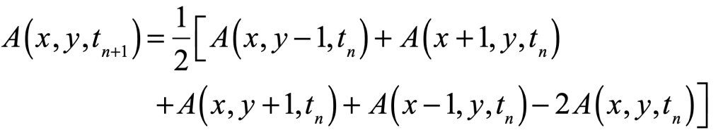
2. J. R. Nagel, A Review and Application of the Finite-Difference Time-Domain Algorithm Applied to the Schrödinger Equation, ACES Journal, Vol. 24, NO. 1, pp. 1-8 (2009)

Quantum Chaos and the Cheshire Cat

Alice’s disturbing adventures in Wonderland tumbled upon her like a string of accidents as she wandered a world of chaos.  Rules were never what they seemed and shifted whenever they wanted.  She even met a cat who grinned ear-to-ear and could disappear entirely, or almost entirely, leaving only its grin.

The vanishing Cheshire Cat reminds us of another famous cat—Arnold’s Cat—that introduced the ideas of stretching and folding of phase-space volumes in non-integrable Hamiltonian systems.  But when Arnold’s Cat becomes a Quantum Cat, a central question remains: What happens to the chaotic behavior of the classical system … does it survive the transition to quantum mechanics?  The answer is surprisingly like the grin of the Cheshire Cat—the cat vanishes, but the grin remains.  In the quantum world of the Cheshire Cat, the grin of the classical cat remains even after the rest of the cat vanished. 

The Cheshire Cat fades away, leaving only its grin, like a fine filament, as classical chaos fades into quantum, leaving behind a quantum scar.

The Quantum Mechanics of Classically Chaotic Systems

The simplest Hamiltonian systems are integrable—they have as many constants of the motion as degrees of freedom.  This holds for quantum systems as well as for classical.  There is also a strong correspondence between classical and quantum systems for the integrable cases—literally the Correspondence Principle—that states that quantum systems at high quantum number approach classical behavior.  Even at low quantum numbers, classical resonances are mirrored by quantum eigenfrequencies that can show highly regular spectra.

But integrable systems are rare—surprisingly rare.  Almost no real-world Hamiltonian system is integrable, because the real world warps the ideal.  No spring can displace indefinitely, and no potential is perfectly quadratic.  There are always real-world non-idealities that destroy one constant of the motion or another, opening the door to chaos.

When classical Hamiltonian systems become chaotic, they don’t do it suddenly.  Almost all transitions to chaos in Hamiltonian systems are gradual.  One of the best examples of this is the KAM theory that starts with invariant action integrals that generate invariant tori in phase space.  As nonintegrable perturbations increase, the tori break up slowly into island chains of stability as chaos infiltrates the separatrixes—first as thin filaments of chaos surrounding the islands—then growing in width to take up more and more of phase space.  Even when chaos is fully developed, small islands of stability can remain—the remnants of stable orbits of the unperturbed system.

When the classical becomes quantum, chaos softens.  Quantum wave functions don’t like to be confined—they spread and they tunnel.  The separatrix of classical chaos—that barrier between regions of phase space—cannot constrain the exponential tails of wave functions.  And the origin of chaos itself—the homoclinic point of the separatrix—gets washed out.  Then the regular orbits of the classical system reassert themselves, and they appear, like the vestige of the Cheshire Cat, as a grin.

The Quantum Circus

The empty stadium is a surprisingly rich dynamical system that has unexpected structure in both the classical and the quantum domain.  Its importance in classical dynamics comes from the fact that its periodic orbits are unstable and its non-periodic orbits are ergodic (filling all available space if given long enough).  The stadium itself is empty so that particles (classical or quantum) are free to propagate between reflections from the perfectly-reflecting walls of the stadium.  The ergodicity comes from the fact that the stadium—like a classic Roman chariot-race stadium, also known as a circus—is not a circle, but has a straight stretch between two half circles.  This simple modification takes the stable orbits of the circle into the unstable orbits of the stadium.

A single classical orbit in a stadium is shown in Fig 1. This is an ergodic orbit that is non-periodic and eventually would fill the entire stadium space. There are other orbits that are nearly periodic, such as one that bounces back and forth vertically between the linear portions, but even this orbit will eventually wander into the circular part of the stadium and then become ergodic. The big quantum-classical question is what happens to these classical orbits when the stadium is shrunk to the nanoscale?

Fig. 1 A classical trajectory in a stadium. It will eventually visit every point, a property known as ergodicity.

Simulating an evolving quantum wavefunction in free space is surprisingly simple. Given a beginning quantum wavefunction A(x,y,t0), the discrete update equation is

Perfect reflection from the boundaries of the stadium are incorporated through imposing a boundary condition that sends the wavefunction to zero. Simple!

A snap-shot of a wavefunction evolving in the stadium is shown in Fig. 2. To see a movie of the time evolution, see my YouTube episode.

Fig. 2 Snapshot of a quantum wavefunction in the stadium. (From YouTube)

The time average of the wavefunction after a long time has passed is shown in Fig. 3. Other than the horizontal nodal line down the center of the stadium, there is little discernible structure or symmetry. This is also true for the mean squared wavefunction shown in Fig. 4, although there is some structure that may be emerging in the semi-circular regions.

Fig. 3 Time-average wavefunction after a long time.
Fig. 4 Time-average of the squared wavefunction after a long time.

On the other hand, for special initial conditions that have a lot of symmetry, something remarkable happens. Fig. 5 shows several mean-squared results for special initial conditions. There is definite structure in these cases that were given the somewhat ugly name “quantum scars” in the 1980’s by Eric Heller who was one of the first to study this phenomenon [1].

Fig. 5 Quantum scars reflect periodic (but unstable) orbits of the classical system. Quantum effects tend to quench chaos and favor regular motion.

One can superpose highly-symmetric classical trajectories onto the figures, as shown in the bottom row. All of these classical orbits go through a high-symmetry point, such as the center of the stadium (on the left image) and through the focal point of the circular mirrors (in the other two images). The astonishing conclusion of this exercise is that the highly-symmetric periodic classical orbits remain behind as quantum scars—like the Cheshire Cat’s grin—when the system is in the quantum realm. The classical orbits that produce quantum scars have the important property of being periodic but unstable. A slight perturbation from the symmetric trajectory causes it to eventually become ergodic (chaotic). These scars are regions with enhanced probability density, what might be termed “quantum trajectories”, but do not show strong interference patterns.

It is important to make the distinction that it is also possible to construct special wavefunctions that are strictly periodic, such as a wave bouncing perfectly vertically between the straight portions. This leads to large-scale interference patterns that are not the same as the quantum scars.

Quantum Chaos versus Laser Speckle

In addition to the bouncing-wave cases that do not strictly produce quantum scars, there is another “neutral” phenomenon that produces interference patterns that look a lot like scars, but are simply the random addition of lots of plane waves with the same wavelength [2]. A snapshot in time of one of these superpositions is shown in Fig. 6. To see how the waves add together, see the YouTube channel episode.

Fig. 6 The sum of 100 randomly oriented plane waves of constant wavelength. (A snapshot from YouTube.)

By David D. Nolte, Aug. 14, 2022


YouTube Video

YouTube Video of Quantum Chaos


References

[1] Heller E J, Bound-state eigenfunctions of classically chaotic hamiltonian-systems – scars of periodic-orbits, Physical Review Letters 53 ,1515 (1984)

[2] Gutzwiller M C, Chaos in classical and quantum mechanics (New York: New York : Springer-Verlag, 1990)

Second Edition of Introduction to Modern Dynamics (Chaos, Networks, Space and Time)

The second edition of Introduction to Modern Dynamics: Chaos, Networks, Space and Time is available from Oxford University Press and Amazon.

Most physics majors will use modern dynamics in their careers: nonlinearity, chaos, network theory, econophysics, game theory, neural nets, geodesic geometry, among many others.

The first edition of Introduction to Modern Dynamics (IMD) was an upper-division junior-level mechanics textbook at the level of Thornton and Marion (Classical Dynamics of Particles and Systems) and Taylor (Classical Mechanics).  IMD helped lead an emerging trend in physics education to update the undergraduate physics curriculum.  Conventional junior-level mechanics courses emphasized Lagrangian and Hamiltonian physics, but notably missing from the classic subjects are modern dynamics topics that most physics majors will use in their careers: nonlinearity, chaos, network theory, econophysics, game theory, neural nets, geodesic geometry, among many others.  These are the topics at the forefront of physics that drive high-tech businesses and start-ups, which is where more than half of all physicists work. IMD introduced these modern topics to junior-level physics majors in an accessible form that allowed them to master the fundamentals to prepare them for the modern world.

The second edition (IMD2) continues that trend by expanding the chapters to include additional material and topics.  It rearranges several of the introductory chapters for improved logical flow and expands them to include key conventional topics that were missing in the first edition (e.g., Lagrange undetermined multipliers and expanded examples of Lagrangian applications).  It is also an opportunity to correct several typographical errors and other errata that students have identified over the past several years.  The second edition also has expanded homework problems.

The goal of IMD2 is to strengthen the sections on conventional topics (that students need to master to take their GREs) to make IMD2 attractive as a mainstream physics textbook for broader adoption at the junior level, while continuing the program of updating the topics and approaches that are relevant for the roles that physicists play in the 21st century.

(New Chapters and Sections highlighted in red.)

New Features in Second Edition:

Second Edition Chapters and Sections

Part 1 Geometric Mechanics

• Expanded development of Lagrangian dynamics

• Lagrange multipliers

• More examples of applications

• Connection to statistical mechanics through the virial theorem

• Greater emphasis on action-angle variables

• The key role of adiabatic invariants

Part 1 Geometric Mechanics

Chapter 1 Physics and Geometry

1.1 State space and dynamical flows

1.2 Coordinate representations

1.3 Coordinate transformation

1.4 Uniformly rotating frames

1.5 Rigid-body motion

Chapter 2 Lagrangian Mechanics

2.1 Calculus of variations

2.2 Lagrangian applications

2.3 Lagrange’s undetermined multipliers

2.4 Conservation laws

2.5 Central force motion

2.6 Virial Theorem

Chapter 3 Hamiltonian Dynamics and Phase Space

3.1 The Hamiltonian function

3.2 Phase space

3.3 Integrable systems and action–angle variables

3.4 Adiabatic invariants

Part 2 Nonlinear Dynamics

• New section on non-autonomous dynamics

• Entire new chapter devoted to Hamiltonian mechanics

• Added importance to Chirikov standard map

• The important KAM theory of “constrained chaos” and solar system stability

• Degeneracy in Hamiltonian chaos

• A short overview of quantum chaos

• Rational resonances and the relation to KAM theory

• Synchronized chaos

Part 2 Nonlinear Dynamics

Chapter 4 Nonlinear Dynamics and Chaos

4.1 One-variable dynamical systems

4.2 Two-variable dynamical systems

4.3 Limit cycles

4.4 Discrete iterative maps

4.5 Three-dimensional state space and chaos

4.6 Non-autonomous (driven) flows

4.7 Fractals and strange attractors

Chapter 5 Hamiltonian Chaos

5.1 Perturbed Hamiltonian systems

5.2 Nonintegrable Hamiltonian systems

5.3 The Chirikov Standard Map

5.4 KAM Theory

5.5 Degeneracy and the web map

5.6 Quantum chaos

Chapter 6 Coupled Oscillators and Synchronization

6.1 Coupled linear oscillators

6.2 Simple models of synchronization

6.3 Rational resonances

6.4 External synchronization

6.5 Synchronization of Chaos

Part 3 Complex Systems

• New emphasis on diffusion on networks

• Epidemic growth on networks

• A new section of game theory in the context of evolutionary dynamics

• A new section on general equilibrium theory in economics

Part 3 Complex Systems

Chapter 7 Network Dynamics

7.1 Network structures

7.2 Random network topologies

7.3 Synchronization on networks

7.4 Diffusion on networks

7.5 Epidemics on networks

Chapter 8 Evolutionary Dynamics

81 Population dynamics

8.2 Virus infection and immune deficiency

8.3 Replicator Dynamics

8.4 Quasi-species

8.5 Game theory and evolutionary stable solutions

Chapter 9 Neurodynamics and Neural Networks

9.1 Neuron structure and function

9.2 Neuron dynamics

9.3 Network nodes: artificial neurons

9.4 Neural network architectures

9.5 Hopfield neural network

9.6 Content-addressable (associative) memory

Chapter 10 Economic Dynamics

10.1 Microeconomics and equilibrium

10.2 Macroeconomics

10.3 Business cycles

10.4 Random walks and stock prices (optional)

Part 4 Relativity and Space–Time

• Relativistic trajectories

• Gravitational waves

Part 4 Relativity and Space–Time

Chapter 11 Metric Spaces and Geodesic Motion

11.1 Manifolds and metric tensors

11.2 Derivative of a tensor

11.3 Geodesic curves in configuration space

11.4 Geodesic motion

Chapter 12 Relativistic Dynamics

12.1 The special theory

12.2 Lorentz transformations

12.3 Metric structure of Minkowski space

12.4 Relativistic trajectories

12.5 Relativistic dynamics

12.6 Linearly accelerating frames (relativistic)

Chapter 13 The General Theory of Relativity and Gravitation

13.1 Riemann curvature tensor

13.2 The Newtonian correspondence

13.3 Einstein’s field equations

13.4 Schwarzschild space–time

13.5 Kinematic consequences of gravity

13.6 The deflection of light by gravity

13.7 The precession of Mercury’s perihelion

13.8 Orbits near a black hole

13.9 Gravitational waves

Synopsis of 2nd Ed. Chapters

Chapter 1. Physics and Geometry (Sample Chapter)

This chapter has been rearranged relative to the 1st edition to provide a more logical flow of the overarching concepts of geometric mechanics that guide the subsequent chapters.  The central role of coordinate transformations is strengthened, as is the material on rigid-body motion with expanded examples.

Chapter 2. Lagrangian Mechanics (Sample Chapter)

Much of the structure and material is retained from the 1st edition while adding two important sections.  The section on applications of Lagrangian mechanics adds many direct examples of the use of Lagrange’s equations of motion.  An additional new section covers the important topic of Lagrange’s undetermined multipliers

Chapter 3. Hamiltonian Dynamics and Phase Space (Sample Chapter)

The importance of Hamiltonian systems and dynamics merits a stand-alone chapter.  The topics from the 1st edition are expanded in this new chapter, including a new section on adiabatic invariants that plays an important role in the development of quantum theory.  Some topics are de-emphasized from the 1st edition, such as general canonical transformations and the symplectic structure of phase space, although the specific transformation to action-angle coordinates is retained and amplified.

Chapter 4. Nonlinear Dynamics and Chaos

The first part of this chapter is retained from the 1st edition with numerous minor corrections and updates of figures.  The second part of the IMD 1st edition, treating Hamiltonian chaos, will be expanded into the new Chapter 5.

Chapter 5. Hamiltonian Chaos

This new stand-alone chapter expands on the last half of Chapter 3 of the IMD 1st edition.  The physical character of Hamiltonian chaos is substantially distinct from dissipative chaos that it deserves its own chapter.  It is also a central topic of interest for complex systems that are either conservative or that have integral invariants, such as our N-body solar system that played such an important role in the history of chaos theory beginning with Poincaré.  The new chapter highlights Poincaré’s homoclinic tangle, illustrated by the Chirikov Standard Map.  The Standard Map is an excellent introduction to KAM theory, which is one of the crowning achievements of the theory of dynamical systems by Komogorov, Arnold and Moser, connecting to deeper aspects of synchronization and rational resonances that drive the structure of systems as diverse as the rotation of the Moon and the rings of Saturn.  This is also a perfect lead-in to the next chapter on synchronization.  An optional section at the end of this chapter briefly discusses quantum chaos to show how Hamiltonian chaos can be extended into the quantum regime.

Chapter 6. Synchronization

This is an updated version of the IMD 1st ed. chapter.  It has a reduced initial section on coupled linear oscillators, retaining the key ideas about linear eigenmodes but removing some irrelevant details in the 1st edition.  A new section is added that defines and emphasizes the importance of quasi-periodicity.  A new section on the synchronization of chaotic oscillators is added.

Chapter 7. Network Dynamics

This chapter rearranges the structure of the chapter from the 1st edition, moving synchronization on networks earlier to connect from the previous chapter.  The section on diffusion and epidemics is moved to the back of the chapter and expanded in the 2nd edition into two separate sections on these topics, adding new material on discrete matrix approaches to continuous dynamics.

Chapter 8. Neurodynamics and Neural Networks

This chapter is retained from the 1st edition with numerous minor corrections and updates of figures.

Chapter 9. Evolutionary Dynamics

Two new sections are added to this chapter.  A section on game theory and evolutionary stable solutions introduces core concepts of evolutionary dynamics that merge well with the other topics of the chapter such as the pay-off matrix and replicator dynamics.  A new section on nearly neutral networks introduces new types of behavior that occur in high-dimensional spaces which are counter intuitive but important for understanding evolutionary drift.

Chapter 10.  Economic Dynamics

This chapter will be significantly updated relative to the 1st edition.  Most of the sections will be rewritten with improved examples and figures.  Three new sections will be added.  The 1st edition section on consumer market competition will be split into two new sections describing the Cournot duopoly and Pareto optimality in one section, and Walras’ Law and general equilibrium theory in another section.  The concept of the Pareto frontier in economics is becoming an important part of biophysical approaches to population dynamics.  In addition, new trends in economics are drawing from general equilibrium theory, first introduced by Walras in the nineteenth century, but now merging with modern ideas of fixed points and stable and unstable manifolds.  A third new section is added on econophysics, highlighting the distinctions that contrast economic dynamics (phase space dynamical approaches to economics) from the emerging field of econophysics (statistical mechanics approaches to economics).

Chapter 11. Metric Spaces and Geodesic Motion

 This chapter is retained from the 1st edition with several minor corrections and updates of figures.

Chapter 12. Relativistic Dynamics

This chapter is retained from the 1st edition with minor corrections and updates of figures.  More examples will be added, such as invariant mass reconstruction.  The connection between relativistic acceleration and Einstein’s equivalence principle will be strengthened.

Chapter 13. The General Theory of Relativity and Gravitation

This chapter is retained from the 1st edition with minor corrections and updates of figures.  A new section will derive the properties of gravitational waves, given the spectacular success of LIGO and the new field of gravitational astronomy.

Homework Problems:

All chapters will have expanded and updated homework problems.  Many of the homework problems from the 1st edition will remain, but the number of problems at the end of each chapter will be nearly doubled, while removing some of the less interesting or problematic problems.

Bibliography

D. D. Nolte, Introduction to Modern Dynamics: Chaos, Networks, Space and Time, 2nd Ed. (Oxford University Press, 2019)