Snell’s Law: The Five-Fold Way

The bending of light rays as they enter a transparent medium—what today is called Snell’s Law—has had a long history of independent discoveries and radically different approaches.  The general problem of refraction was known to the Greeks in the first century AD, and it was later discussed by the Arabic scholar Alhazan.  Ibn Sahl in Bagdad in 984 AD was the first to put an accurate equation to the phenomenon.  Thomas Harriott in England discussed the problem with Johannes Kepler in 1602, unaware of the work by Ibn Sahl.  Willebrord Snellius (1580–1626) in the Netherlands derived the equation for refraction in 1621, but did not publish it, though it was known to Christian Huygens (1629 – 1695).  René Descartes (1596 – 1650), unaware of Snellius’ work, derived the law in his Dioptrics, using his newly-invented coordinate geometry.  Christiaan Huygens, in his Traité de la Lumière in 1678, derived the law yet again, this time using his principle of secondary waves, though he acknowledged the prior work of Snellius, permanently cementing the shortened name “Snell” to the law of refraction. Snell’s Law is a special case of the Eikonal Equation and is useful to calculate the caustic envelope of rays transmitted through undulating surfaces.

Through this history and beyond, there have been many approaches to deriving Snell’s Law.  Some used ideas of momentum, while others used principles of waves.  Today, there are roughly five different ways to derive Snell’s law.  These are:

            1) Huygens’ Principle,

            2) Fermat’s Principle,

            3) Wavefront Continuity

            4) Plane-wave Boundary Conditions, and

            5) Photon Momentum Conservation.

The approaches differ in detail, but they fall into two rough categories:  the first two fall under minimization or extremum principles, and the last three fall under continuity or conservation principles.

Snell’s Law: Huygens’ Principle

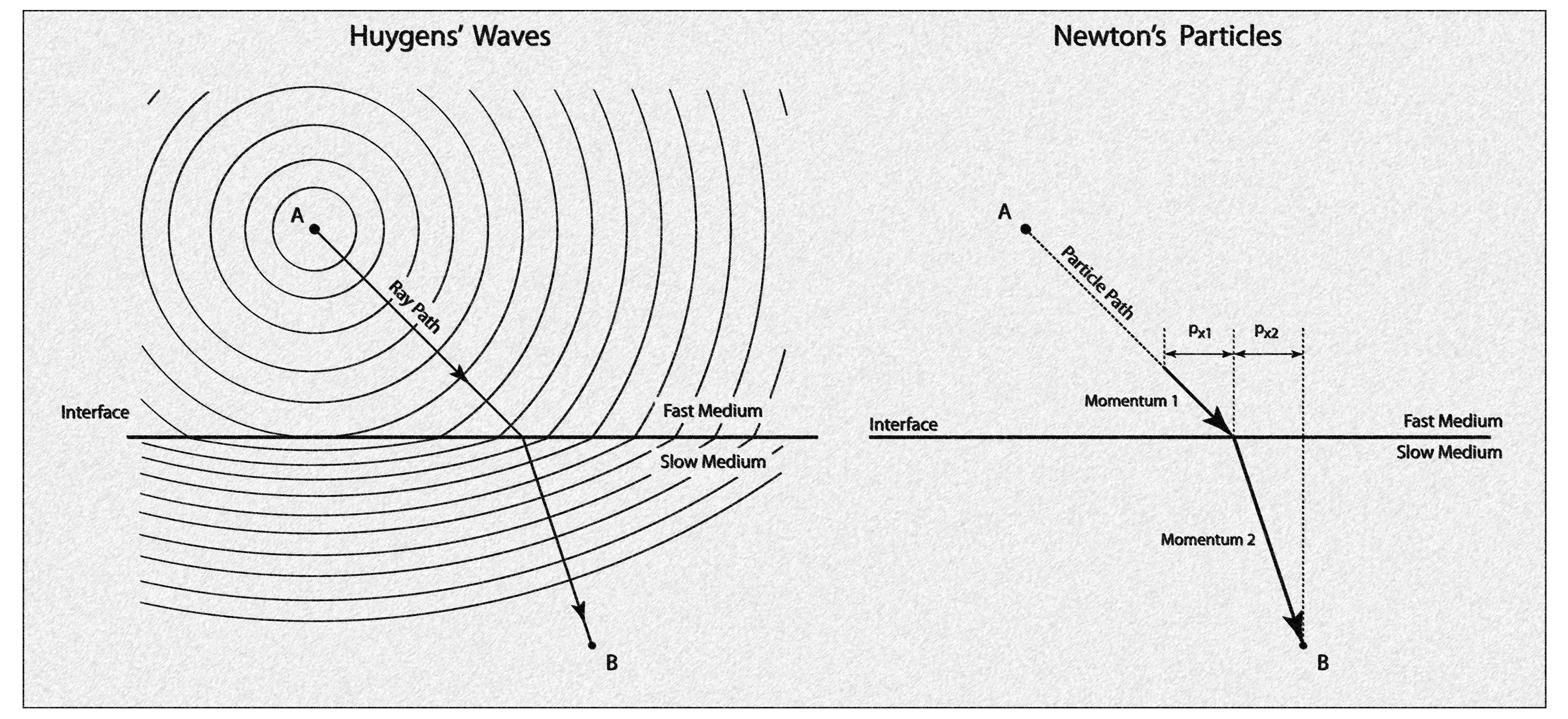
Huygens’ principle, published in 1687, states that every point on a wavefront serves as the source of a spherical secondary wave.  This was one of the first wave principles ever proposed for light (Robert Hooke had suggested that light had wavelike character based on his observations of colors in thin films) yet remains amazingly powerful even today.  It can be used not only to derive Snell’s law but also properties of light scattering and diffraction.  Huygens’ principle is a form of minimization principle:  it finds the direction of propagation (for a spherically expanding wavefront from a point where a ray strikes a surface) that yields a minimum angle (tangent to the surface) relative to a second source.  Finding the tangent to the spherical surface is a minimization problem and yields Snell’s Law.

Fig. 1 Huygens’ principle.

            The use of Huygen’s principle for the derivation of Snell’s Law is shown in Fig. 1.  Two parallel incoming rays strike a surface a distance d apart.  The first point emits a secondary spherical wave into the second medium.  The wavefront propagates at a speed of v2 relative to the speed in the first medium of v1.  In the diagram, the propagation distance over the distance d is equal to the sine of the angle

Solving for d and equating the two equations gives

The speed depends on the refractive index as

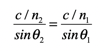
which leads to Snell’s Law:

Snell’s Law: Fermat’s Principle

Fermat’s principle of least time is a direct minimization problem that finds the least time it takes light to propagate from one point to another.  One of the central questions about Fermat’s principle is: why does it work?  Why is the path of least time the path light needs to take?  I’ll answer that question after we do the derivation.  The configuration of the problem is shown in Fig. 2.

Fig. 2 Fermat’s principle of least time and Feynman’s principle of stationary action leading to maximum constructive interference.

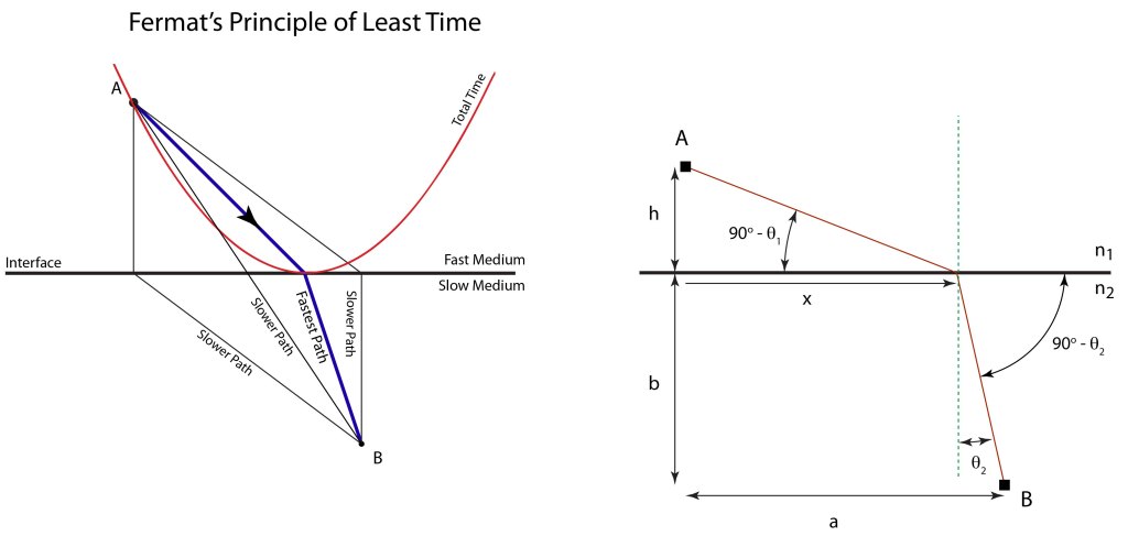
Consider a source point A and a destination point B.  Light travels in a strait line in each medium, deflecting at the point x on the figure.  The speed in medium 1 is c/n1, and the speed in medium 2 is c/n2.  What position x provides the minimum time?

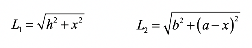
The distances from A to x, and from x to B are, respectively:

The total time is

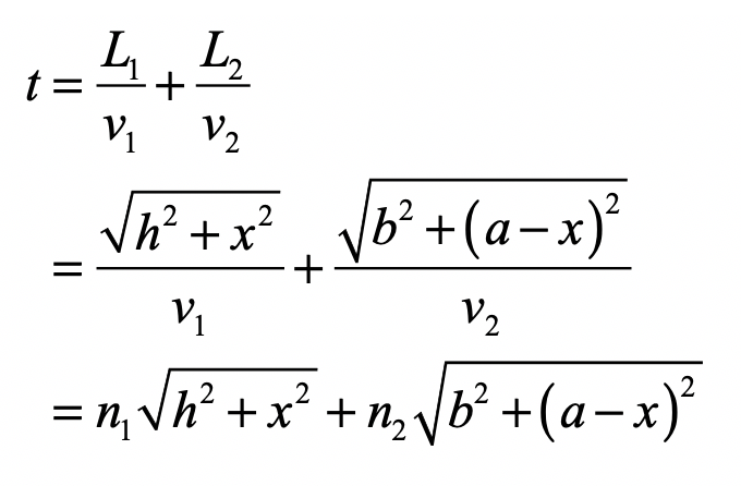
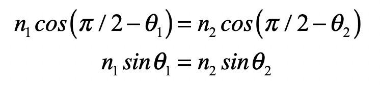
Minimize this expression by taking the derivative of the time relative to the position x and setting the result to zero

Converting the cosines to sines yields Snell’s Law

Fermat’s principle of least time can be explained in terms of wave interference.  If we think of all paths being taken by propagating waves, then those waves that take paths that differ only a little from the optimum path still interfere constructively.  This is the principle of stationarity and is related to the principle of least action.  The time minimizes a quadratic expression that deviates from the minimum only in second order (shown in the right part of Fig. 2).  Therefore, all “nearby” paths interfere constructively, while paths that are farther away begin to interfere destructively.  Therefore, the path of least time is also the path of stationary time and hence stationary optical path length and hence the path of maximum constructive interference.  This is the actual path taken by the wave—and the light.

Snell’s Law: Wavefront Continuity

When a wave passes across an interface between two transparent media the phase of the wave remains continuous.  This continuity of phase provides a way to derive Snell’s Law.  Consider Fig. 3.  A plane wave with wavelength l1 is incident from medium 1 on an interface with medium 2 in which the wavelength is l2.  The wavefronts remain continuous, but they are “kinked” at the interface. 

Fig. 3 Wavefront continuity.

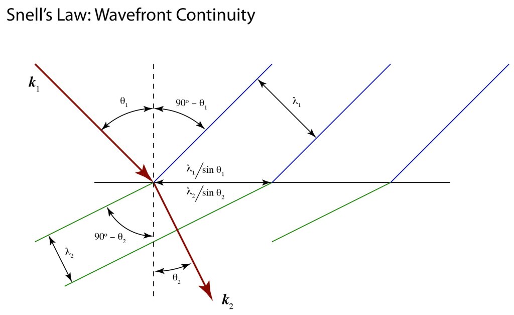
The waves in medium 1 and medium 2 share the part of the interface between wavefronts.  This distance is

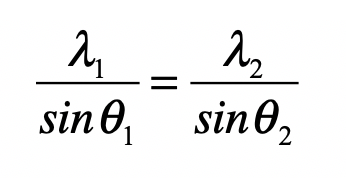
The wavelengths in the two media are related to the refractive index through

where l0 is the free-space wavelength.  Plugging these into the first expression yields

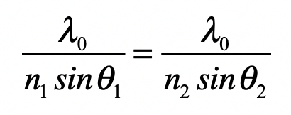
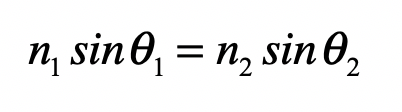
which relates the denominators through Snell’s Law

Snell’s Law: Plane-Wave Boundary Condition

Maxwell’s four equations in integral form can each be applied to the planar interface between two refractive media.

Fig. 4 Electromagnetic boundary conditions leading to phase-matching at the planar interface.

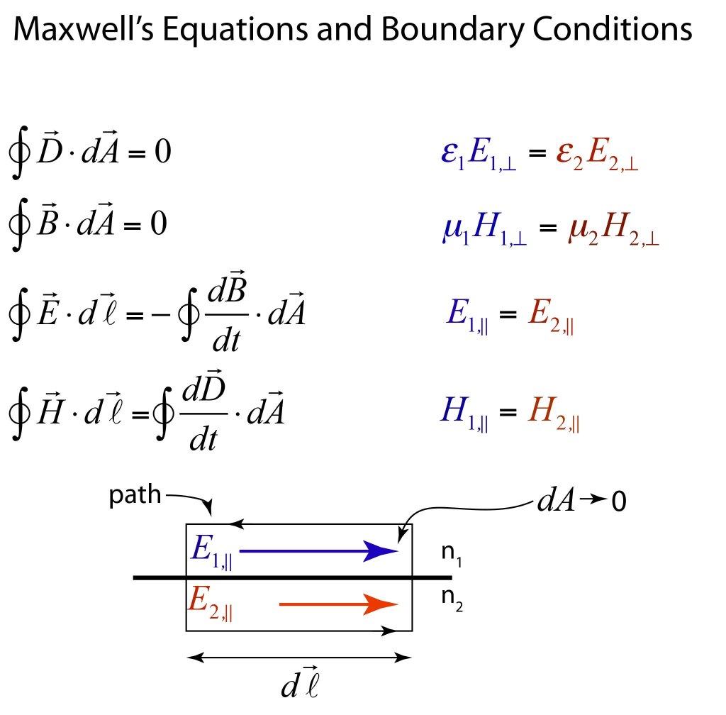
All four boundary conditions can be written as

where i, r and t stand for incident, reflected and transmitted. The only way this condition can be true for all possible values of the fields is if the phases of the wave terms are all the same (phase-matching), namely

which in turn guarantees that the transverse projection of the k-vector is continuous across the interface

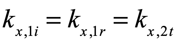
and the transverse components (projections) are

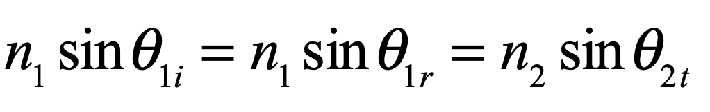
where the last line states both Snell’s law of refraction and the law of reflection. Therefore, the general wave boundary condition leads immediately to Snell’s Law.

Snell’s Law: Momentum Conservation

Going from Maxwell’s equations for classical fields to photons keeps the same mathematical form for the transverse components for the k-vectors, but now interprets them in a different manner.  Where before there was a requirement for phase-matching the classical waves at the interface, in the photon picture the transverse k-vector becomes the transverse momentum through de Broglie’s equation

Therefore, continuity of the transverse k-vector is interpreted as conservation of transverse momentum of the photon across the interface.  In the figure the second medium is denser with a larger refractive index n2 > n1.  Hence, the momentum of the photon in the second medium is larger while keeping the transverse momentum projection the same.  This simple interpretation gives the same mathematical form as the previous derivation using classical boundary conditions, namely

which is again Snell’s law and the law of reflection.

Fig. 5 Conservation of transverse photon momentum.

Recap

Snell’s Law has an eerie habit of springing from almost any statement that can be made about a dielectric interface. It yields the path of least time, tracks the path of maximum constructive interference, produces wavefronts that are extremally tangent to wavefronts, connects continuous wavefronts across the interface, conserves transverse momentum, and guarantees phase matching. These all sound very different, yet all lead to the same simple law of Snellius and Ibn Sahl.

This is deep physics!


New from Oxford Press: The History of Optical Interferometry (Summer 2023)

Wave-Particle Duality and Hamilton’s Physics

Wave-particle duality was one of the greatest early challenges to quantum physics, partially clarified by Bohr’s Principle of Complementarity, but never easily grasped even today.  Yet long before Einstein proposed the indivisible quantum  of light (later to be called the photon by the chemist Gilbert Lewis), wave-particle duality was firmly embedded in the foundations of the classical physics of mechanics.

Light led the way to mechanics more than once in the history of physics.


Willebrord Snel van Royen

The Dutch physicist Willebrord Snel van Royen in 1621 derived an accurate mathematical description of the refraction of beams of light at a material interface in terms of sine functions, but he did not publish.  Fifteen years later, as Descartes was looking for an example to illustrate his new method of analytic geometry, he discovered the same law, unaware of Snel’s prior work.  In France the law is known as the Law of Descartes.  In the Netherlands (and much of the rest of the world) it is known as Snell’s Law.  Both Snell and Descartes based their work on Newton’s corpuscles of light.  The brilliant Fermat adopted corpuscles when he developed his principle of least time to explain the law of Descartes in 1662.  Yet Fermat was forced to assume that the corpuscles traveled slower in the denser material even though it was generally accepted that light should travel faster in denser media, just as sound did.  Seventy-five years later, Maupertuis continued the tradition when he developed his principle of least action and applied it to light corpuscles traveling faster through denser media, just as Descartes had prescribed.

HuygensParticle-02

The wave view of Snell’s Law (on the left). The source resides in the medium with higher speed. As the wave fronts impinge on the interface to a medium with lower speed, the wave fronts in the slower medium flatten out, causing the ray perpendicular to the wave fronts to tilt downwards. The particle view of Snell’s Law (on the right). The momentum of the particle in the second medium is larger than in the first, but the transverse components of the momentum (the x-components) are conserved, causing a tilt downwards of the particle’s direction as it crosses the interface. [i]

Maupertuis’ paper applying the principle of least action to the law of Descartes was a critical juncture in the development of dynamics.  His assumption of faster speeds in denser material was wrong, but he got the right answer because of the way he defined action for light.  Encouraged by the success of his (incorrect) theory, Maupertuis extended the principle of least action to mechanical systems, and this time used the right theory to get the right answers.  Despite Maupertuis’ misguided aspirations to become a physicist of equal stature to Newton, he was no mathematician, and he welcomed (and  somewhat appropriated) the contributions of Leonid Euler on the topic, who established the mathematical foundations for the principle of least action.  This work, in turn, attracted the attention of the Italian mathematician Lagrange, who developed a general new approach (Lagrangian mechanics) to mechanical systems that included the principle of least action as a direct consequence of his equations of motion.  This was the first time that light led the way to classical mechanics.  A hundred years after Maupertuis, it was time again for light to lead to the way to a deeper mechanics known as Hamiltonian mechanics.

Young Hamilton

William Rowland Hamilton (1805—1865) was a prodigy as a boy who knew parts of thirteen languages by the time he was thirteen years old. These were Greek, Latin, Hebrew, Syriac, Persian, Arabic, Sanskrit, Hindoostanee, Malay, French, Italian, Spanish, and German. In 1823 he entered Trinity College of Dublin University to study science. In his second and third years, he won the University’s top prizes for Greek and for mathematical physics, a run which may have extended to his fourth year—but he was offered the position of Andrew’s Professor of Astronomy at Dublin and Royal Astronomer of Ireland—not to be turned down at the early age of 21.

Hamilton1

Title of Hamilton’s first paper on his characteristic function as a new method that applied his theory from optics to the theory of mechanics, including Lagrangian mechanics as a special case.

His research into mathematical physics  concentrated on the theory of rays of light. Augustin-Jean Fresnel (1788—1827) had recently passed away, leaving behind a wave theory of light that provided a starting point for many effects in optical science, but which lacked broader generality. Hamilton developed a rigorous mathematical framework that could be applied to optical phenomena of the most general nature. This led to his theory of the Characteristic Function, based on principles of the variational calculus of Euler and Lagrange, that predicted the refraction of rays of light, like trajectories, as they passed through different media or across boundaries. In 1832 Hamilton predicted a phenomenon called conical refraction, which would cause a single ray of light entering a biaxial crystal to refract into a luminous cone.

Mathematical physics of that day typically followed experimental science. There were so many observed phenomena in so many fields that demanded explanation, that the general task of the mathematical physicist was to explain phenomena using basic principles followed by mathematical analysis. It was rare for the process to work the other way, for a theorist to predict a phenomenon never before observed. Today we take this as very normal. Einstein’s fame was primed by his prediction of the bending of light by gravity—but only after the observation of the effect by Eddington four years later was Einstein thrust onto the world stage. The same thing happened to Hamilton when his friend Humphrey Lloyd observed conical refraction, just as Hamilton had predicted. After that, Hamilton was revered as one of the most ingenious scientists of his day.

Following the success of conical refraction, Hamilton turned from optics to pursue a striking correspondence he had noted in his Characteristic Function that applied to mechanical trajectories as well as it did to rays of light. In 1834 and 1835 he published two papers On a General Method in Mechanics( I and II)[ii], in which he reworked the theory of Lagrange by beginning with the principle of varying action, which is now known as Hamilton’s Principle. Hamilton’s principle is related to Maupertuis’ principle of least action, but it was more rigorous and a more general approach to derive the Euler-Lagrange equations.  Hamilton’s Principal Function allowed the trajectories of particles to be calculated in complicated situations that were challenging for a direct solution by Lagrange’s equations.

The importance that these two papers had on the future development of physics would not be clear until 1842 when Carl Gustav Jacob Jacobi helped to interpret them and augment them, turning them into a methodology for solving dynamical problems. Today, the Hamiltonian approach to dynamics is central to all of physics, and thousands of physicists around the world mention his name every day, possibly more often than they mention Einstein’s.

[i] Reprinted from D. D. Nolte, Galileo Unbound: A Path Across Life, the Universe and Everything (Oxford, 2018)

[ii] W. R. Hamilton, “On a general method in dynamics I,” Phil. Trans. Roy. Soc., pp. 247-308, 1834; W. R. Hamilton, “On a general method in dynamics II,” Phil. Trans. Roy. Soc., pp. 95-144, 1835.

Huygens’ Tautochrone

In February of 1662, Pierre de Fermat wrote a paper Synthesis ad refractiones that explained Descartes-Snell’s Law of light refraction by finding the least time it took for light to travel between two points. This famous approach is now known as Fermat’s principle, and it motivated other searches for minimum principles. A few years earlier, in 1656, Christiaan Huygens had invented the pendulum clock [1], and he began a ten-year study of the physics of the pendulum. He was well aware that the pendulum clock does not keep exact time—as the pendulum swings wider, the period of oscillation slows down. He began to search for a path of the pendular mass that would keep the period the same (and make pendulum clocks more accurate), and he discovered a trajectory along which a mass would arrive at the same position in the same time no matter where it was released on the curve. That such a curve could exist was truly remarkable, and it promised to make highly accurate time pieces.

It made minimization problems a familiar part of physics—they became part of the mindset, leading ultimately to the principle of least action.

This curve is known as a tautochrone (literally: same or equal time in Greek) and Huygens provided a geometric proof in his Horologium Oscillatorium sive de motu pendulorum (1673) that the curve was a cycloid [2]. A cycloid is the curve traced by a point on the rim of a circular wheel as the wheel rolls without slipping along a straight line. Huygens invented such a pendulum in which the mass executed a cycloid curve. It was a mass on a flexible yet inelastic string that partially wrapped itself around a solid bumper on each half swing. In principle, whether the pendulum swung gently, or through large displacements, the time would be the same. Unfortunately, friction along the contact of the string with the bumper prevented the pendulum from achieving this goal, and the tautochronic pendulum did not catch on.

HuygensIsochron

Fig. 1 Huygens’ isochronous pendulum.  The time it takes the pendulum bob to follow the cycloid arc is independent of the pendulum’s amplitude, unlike for the circular arc, as the pendulum slows down for larger excursions.

The solution of the tautochrone curve of equal time led naturally to a search for the curve of least time, known as the brachistochrone curve for a particle subject to gravity, like a bead sliding on a frictionless wire between two points. Johann Bernoulli published a challenge to find the brachistochrone in 1696 in the scientific journal Acta Eruditorum that had been founded in 1682 by Leibniz in Germany in collaboration with Otto Mencke. Leibniz envisioned the journal to be a place where new ideas in the natural sciences and mathematics could be published and disseminated rapidly, and it included letters and commentaries, acting as a communication hub to help establish a community of scholars across Europe. In reality, it was the continental response to the Proceedings of the Royal Society in England.  Naturally, the Acta and the Proceedings would later take partisan sides in the priority dispute between Leibniz and Newton for the development of the calculus.

When Bernoulli published his brachistochrone challenge in the June issue of 1696, it was read immediately by the leading mathematicians of the day, many of whom took up the challenge and replied. The problem was solved and published in the May 1697 issue of the Acta by no less than five correspondents, including Johann Bernoulli, Jakob Bernoulli (Johann’s brother), Isaac Newton, Gottfried Leibniz and Ehrenfried Walther von Tschirnhaus. Each of them varied in their approaches, but all found the same solution. Johann and Jakob each considered the problem as the path of a light beam in a medium whose speed varied with depth. Just as in the tautochrone, the solved curve was a cycloid. The path of fastest time always started with a vertical path that allowed the fastest acceleration, and the point of greatest depth always was at the point of greatest horizontal speed.

The brachistrochrone problem led to the invention of the variational calculus, with first steps by Jakob Bernoulli and later more rigorous approaches by Euler.  However, its real importance is that it made minimization problems a familiar part of physics—they became part of the mindset, leading ultimately to the principle of least action.

Mathematical Description of the Tautochrone Curve

If the length of the pendulum is L, the position coordinates (relative to the cusp of the cycloid) are

where the angle θ is between the straight section of the string and the vertical and depends on time as

for a maximum angle θ0. The angular frequency of the isochronous pendulum is given by the standard expression for a small-amplitude pendulum as

For small-angle oscillations, the tautochrone and the conventional pendulum have the same periods and amplitudes. The difference is that the tautochrone has that same period regardless of the amplitude, so no approximation is needed.

Huygens’ proof of the tautochrone curve was made geometrically without the use of calculus, requiring almost 18 pages and 16 figures.

The modern proof (due to Euler) takes only a few lines of calculus. All that is needed is to recognize that the equation of motion of the pendulum bob along its path of length s should be that of a simple-harmonic oscillator

because a simple harmonic oscillator always oscillates at the same frequency regardless of amplitude. Of course, a simple pendulum is not a simple harmonic oscillator because it becomes nonlinear and slows down for large amplitudes. The right-hand-side is the standard force on the bob given by the gradient of the potential energy along the curve

yielding the simple differential equation

which is integrated to give a quadratic dependence of height on path length

To get an equation for the curve itself, plug this back in to the differential equation and square it to give

Euler recognized this as the differential equation of a cycloid

Notes

[1] Galileo conceived the pendulum clock in 1641, and his son Vincenzo started construction, but it was never finished.  Huygens submitted and received a patent in 1657 for a practical escape mechanism on pendulum clocks that is still used today.

[2] Huygens, Christiaan; Blackwell,, Richard J., trans. (1986). Horologium Oscillatorium (The Pendulum Clock, or Geometrical demonstrations concerning the motion of pendula as applied to clocks). Ames, Iowa: Iowa State University Press