
We are at War! That may sound like a cliche, but more people in the United States may die over the next year from COVID-19 than US soldiers have died in all the wars ever fought in US history. It is a war against an invasion by an alien species that has no remorse and gives no quarter. In this war, one of our gravest enemies, beyond the virus, is misinformation. The Internet floods our attention with half-baked half-truths. There may even be foreign powers that see this time of crisis as an opportunity to sow fear through disinformation to divide the country.
Because of the bifurcation physics of the SIR model of COVID-19, small changes in personal behavior (if everyone participates) can literally save Millions of lives!
At such times, physicists may be tapped to help the war effort. This is because physicists have unique skill sets that help us see through the distractions of details to get to the essence of the problem. Our solutions are often back-of-the-envelope, but that is their strength. We can see zeroth-order results stripped bare of all the obfuscating minutia.
One way physicists can help in this war is to shed light on how infections percolate through a population and to provide estimates on the numbers involved. Perhaps most importantly, we can highlight what actions ordinary citizens can take that best guard against the worst-case scenarios of the pandemic. The zeroth-oder solutions may not say anything new that the experts don’t already know, but it may help spread the word of why such simple actions as shelter-in-place may save millions of lives.
The SIR Model of Infection
One of the simplest models for infection is the so-called SIR model that stands for Susceptible-Infected-Removed. This model is an averaged model (or a mean-field model) that disregards the fundamental network structure of human interactions and considers only averages. The dynamical flow equations are very simple
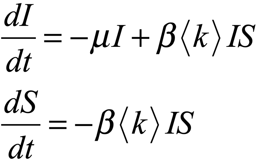
where I is the infected fraction of the population, and S is the susceptible fraction of the population. The coefficient μ is the rate at which patients recover or die, <k> is the average number of “links” to others, and β is the infection probability per link per day. The total population fraction is give by the constraint
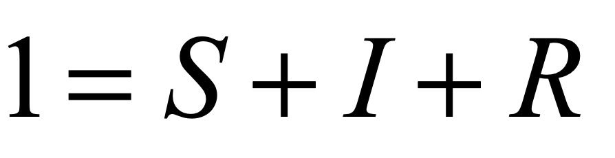
where R is the removed population, most of whom will be recovered, but some fraction will have passed away. The number of deaths is
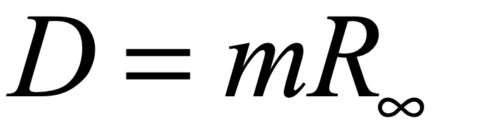
where m is the mortality rate, and Rinf is the longterm removed fraction of the population after the infection has run its course.
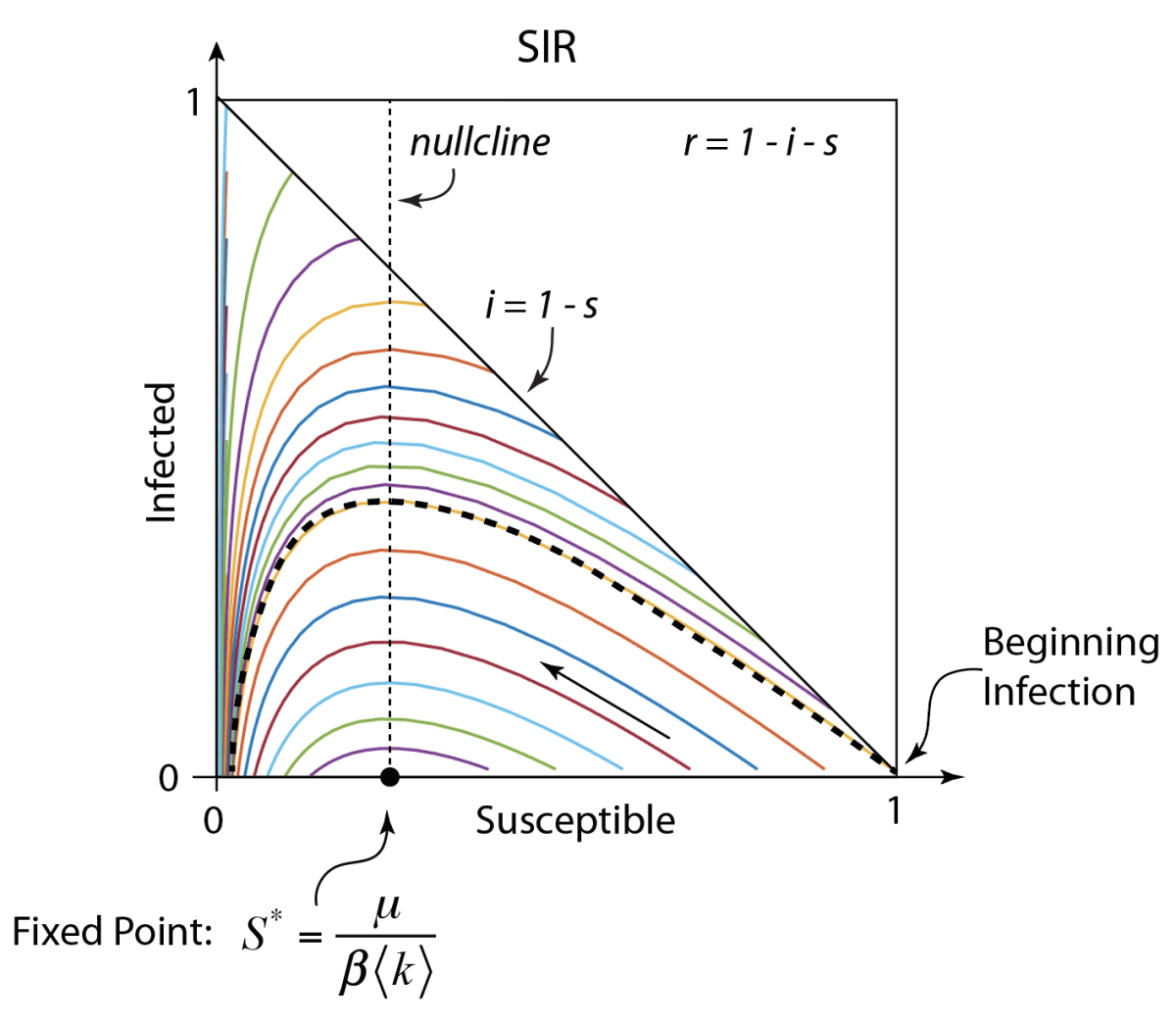
The nullclines, the curves along which the time derivatives vanish, are
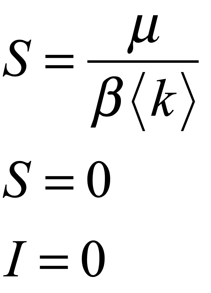
Where the first nullcline intersects the third nullcline is the only fixed point of this simple model
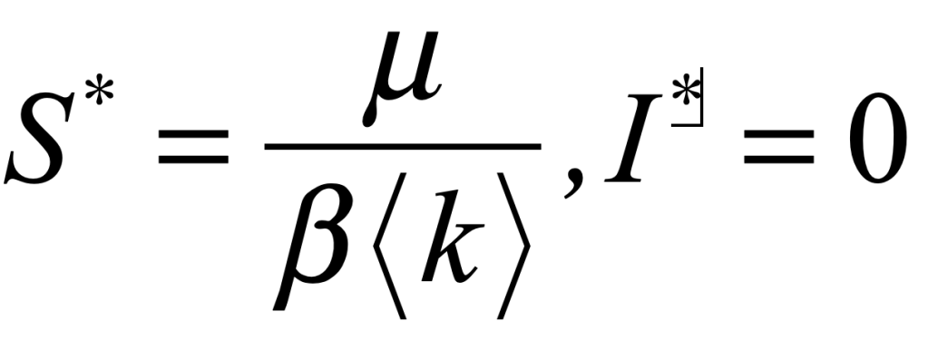
The phase space of the SIR flow is shown in Fig. 1 plotted as the infected fraction as a function of the susceptible fraction. The diagonal is the set of initial conditions where R = 0. Each initial condition on the diagonal produces a dynamical trajectory. The dashed trajectory that starts at (1,0) is the trajectory for a new disease infecting a fully susceptible population. The trajectories terminate on the I = 0 axis at long times when the infection dies out. In this model, there is always a fraction of the population who never get the disease, not through unusual immunity, but through sheer luck.

The key to understanding the scale of the pandemic is the susceptible fraction at the fixed point S*. For the parameters chosen to plot Fig. 1, the value of S* is 1/4, or β<k> = 4μ. It is the high value of the infection rate β<k> relative to the decay rate of the infection μ that allows a large fraction of the population to become infected. As the infection rate gets smaller, the fixed point S* moves towards unity on the horizontal axis, and less of the population is infected.
As soon as S* exceeds unity, for the condition
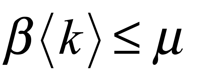
then the infection cannot grow exponentially and will decay away without infecting an appreciable fraction of the population. This condition represents a bifurcation in the infection dynamics. It means that if the infection rate can be reduced below the recovery rate, then the pandemic fades away. (It is important to point out that the R0 of a network model (the number of people each infected person infects) is analogous to the inverse of S*. When R0 > 1 then the infection spreads, just as when S* < 1, and vice versa.)
This bifurcation condition makes the strategy for fighting the pandemic clear. The parameter μ is fixed by the virus and cannot be altered. But the infection probability per day per social link, β, can be reduced by clean hygiene:
- Don’t shake hands
- Wash your hands often and thoroughly
- Don’t touch your face
- Cover your cough or sneeze in your elbow
- Wear disposable gloves
- Wipe down touched surfaces with disinfectants
And the number of contacts per person, <k>, can be reduced by social distancing:
- No large gatherings
- Stand away from others
- Shelter-in-place
- Self quarantine
The big question is: can the infection rate be reduced below the recovery rate through the actions of clean hygiene and social distancing? If there is a chance that it can, then literally millions of lives can be saved. So let’s take a look at COVID-19.
The COVID-19 Pandemic
To get a handle on modeling the COVID-19 pandemic using the (very simplistic) SIR model, one key parameter is the average number of people you are connected to, represented by <k>. These are not necessarily the people in your social network, but also includes people who may touch a surface you touched earlier, or who touched a surface you later touch yourself. It also includes anyone in your proximity who has coughed or sneezed in the past few minutes. The number of people in your network is a topic of keen current interest, but is surprisingly hard to pin down. For the sake of this model, I will take the number <k> = 50 as a nominal number. This is probably too small, but it is compensated by the probability of infection given by a factor r and by the number of days that an individual is infectious.
The spread is helped when infectious people go about their normal lives infecting others. But if a fraction of the population self quarantines, especially after they “may” have been exposed, then the effective number of infectious dinf days per person can be decreased. A rough equation that captures this is
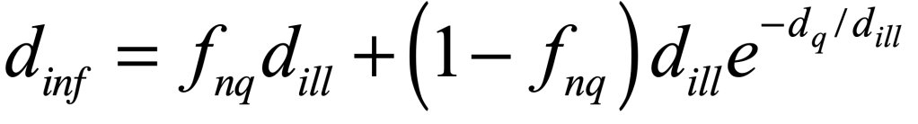
where fnq is the fraction of the population that does NOT self quarantine, dill is the mean number of days a person is ill (and infectious), and dq is the number of days quarantined. This number of infectious days goes into the parameter β.
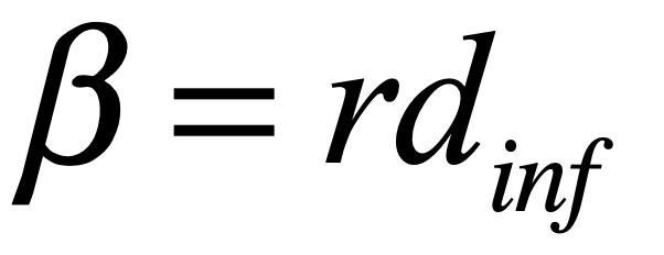
where r = 0.0002 infections per link per day2 , which is a very rough estimate of the coefficient for COVID-19.
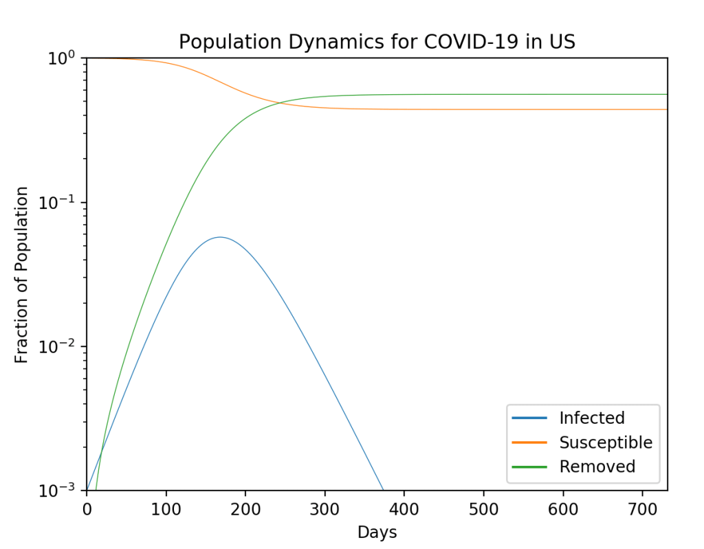
It is clear why shelter-in-place can be so effective, especially if the number of days quarantined is equal to the number of days a person is ill. The infection could literally die out if enough people self quarantine by pushing the critical value S* above the bifurcation threshold. However, it is much more likely that large fractions of people will continue to move about. A simulation of the “wave” that passes through the US is shown in Fig. 2 (see the Python code in the section below for parameters). In this example, 60% of the population does NOT self quarantine. The wave peaks approximately 150 days after the establishment of community spread.
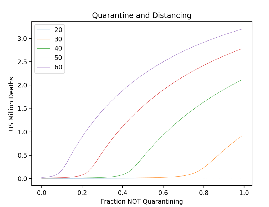
In addition to shelter-in-place, social distancing can have a strong effect on the disease spread. Fig. 3 shows the number of US deaths as a function of the fraction of the population who do NOT self-quarantine for a series of average connections <k>. The bifurcation effect is clear in this graph. For instance, if <k> = 50 is a nominal value, then if 85% of the population would shelter-in-place for 14 days, then the disease would fall below threshold and only a small number of deaths would occur. But if that connection number can be dropped even to <k> = 40, then only 60% would need to shelter-in-place to avoid the pandemic. By contrast, if 80% of the people don’t self-quarantine, and if <k> = 40, then there could be 2 Million deaths in the US by the time the disease has run its course.
Because of the bifurcation physics of this SIR model of COVID-19, small changes in personal behavior (if everyone participates) can literally save Millions of lives!
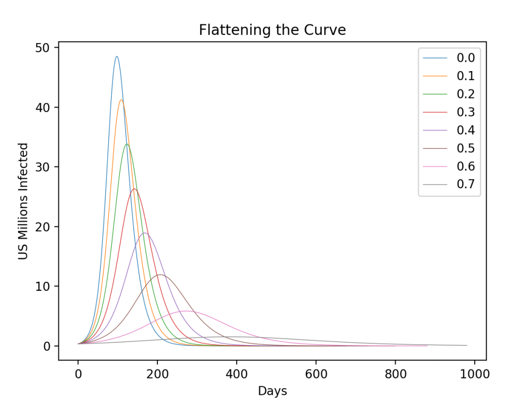
There has been a lot said about “flattening the curve”, which is shown in Fig. 4. There are two ways that flattening the curve saves overall lives: 1) it keeps the numbers below the threshold capacity of hospitals; and 2) it decreases the total number infected and hence decreases the total dead. When the number of critical patients exceeds hospital capacity, the mortality rate increases. This is being seen in Italy where the hospitals have been overwhelmed and the mortality rate has risen from a baseline of 1% or 2% to as large as 8%. Flattening the curve is achieved by sheltering in place, personal hygiene and other forms of social distancing. The figure shows a family of curves for different fractions of the total population who shelter in place for 14 days. If more than 70% of the population shelters in place for 14 days, then the curve not only flattens … it disappears!
Python Code: SIR.py
#!/usr/bin/env python3
# -*- coding: utf-8 -*-
"""
SIR.py
Created on Sat March 21 2020
@author: nolte
D. D. Nolte, Introduction to Modern Dynamics: Chaos, Networks, Space and Time, 2nd ed. (Oxford,2019)
"""

import numpy as np
from scipy import integrate
from matplotlib import pyplot as plt

plt.close('all')

print(' ')
print('SIR.py')

def solve_flow(param,max_time=1000.0):

    def flow_deriv(x_y,tspan,mu,betap):
        x, y = x_y

        return [-mu*x + betap*x*y,-betap*x*y]

    x0 = [del1, del2]

    # Solve for the trajectories
    t = np.linspace(0, int(tlim), int(250*tlim))
    x_t = integrate.odeint(flow_deriv, x0, t, param)


    return t, x_t


r = 0.0002    # 0.0002
k = 50        # connections  50
dill = 14     # days ill 14
dpq = 14      # days shelter in place 14
fnq = 0.6     # fraction NOT sheltering in place
mr0 = 0.01    # mortality rate
mr1 = 0.03     # extra mortality rate if exceeding hospital capacity
P = 330       # population of US in Millions
HC = 0.003    # hospital capacity

dinf = fnq*dill + (1-fnq)*np.exp(-dpq/dill)*dill;

betap = r*k*dinf;
mu = 1/dill;

print('beta = ',betap)
print('dinf = ',dinf)
print('beta/mu = ',betap/mu)

del1 = .001         # infected
del2 = 1-del1       # susceptible

tlim = np.log(P*1e6/del1)/betap + 50/betap

param = (mu, betap)    # flow parameters

t, y = solve_flow(param)
I = y[:,0]
S = y[:,1]
R = 1 - I - S

plt.figure(1)
lines = plt.semilogy(t,I,t,S,t,R)
plt.ylim([0.001,1])
plt.xlim([0,tlim])
plt.legend(('Infected','Susceptible','Removed'))
plt.setp(lines, linewidth=0.5)
plt.xlabel('Days')
plt.ylabel('Fraction of Population')
plt.title('Population Dynamics for COVID-19 in US')
plt.show()

mr = mr0 + mr1*(0.2*np.max(I)-HC)*np.heaviside(0.2*np.max(I),HC)
Dead = mr*P*R[R.size-1]
print('US Dead = ',Dead)

D = np.zeros(shape=(100,))
x = np.zeros(shape=(100,))
for kloop in range(0,5):
    for floop in range(0,100):

        fnq = floop/100

        dinf = fnq*dill + (1-fnq)*np.exp(-dpq/dill)*dill;

        k = 20 + kloop*10
        betap = r*k*dinf

        tlim = np.log(P*1e6/del1)/betap + 50/betap

        param = (mu, betap)    # flow parameters

        t, y = solve_flow(param)
        I = y[:,0]
        S = y[:,1]
        R = 1 - I - S

        mr = mr0 + mr1*(0.2*np.max(I)-HC)*np.heaviside(0.2*np.max(I),HC)

        D[floop] = mr*P*R[R.size-1]
        x[floop] = fnq

    plt.figure(2)
    lines2 = plt.plot(x,D)
    plt.setp(lines2, linewidth=0.5)

plt.ylabel('US Million Deaths')
plt.xlabel('Fraction NOT Quarantining')
plt.title('Quarantine and Distancing')
plt.legend(('20','30','40','50','60','70'))
plt.show()


label = np.zeros(shape=(9,))
for floop in range(0,8):

    fq = floop/10.0

    dinf = (1-fq)*dill + fq*np.exp(-dpq/dill)*dill;

    k = 50
    betap = r*k*dinf

    tlim = np.log(P*1e6/del1)/betap + 50/betap

    param = (mu, betap)    # flow parameters

    t, y = solve_flow(param)
    I = y[:,0]
    S = y[:,1]
    R = 1 - I - S

    plt.figure(3)
    lines2 = plt.plot(t,I*P)
    plt.setp(lines2, linewidth=0.5)
    label[floop]=fq

plt.legend(label)
plt.ylabel('US Millions Infected')
plt.xlabel('Days')
plt.title('Flattening the Curve')
You can run this Python code yourself and explore the effects of changing the parameters. For instance, the mortality rate is modeled to increase when the number of hospital beds is exceeded by the number of critical patients. This coefficient is not well known and hence can be explored numerically. Also, the infection rate r is not known well, nor the average number of connections per person. The effect of longer quarantines can also be tested relative to the fraction who do not quarantine at all. Because of the bifurcation physics of the disease model, large changes in dynamics can occur for small changes in parameters when the dynamics are near the bifurcation threshold.
Caveats and Disclaimers
This SIR model of COVID-19 is an extremely rough tool that should not be taken too literally. It can be used to explore ideas about the general effect of days quarantined, or changes in the number of social contacts, but should not be confused with the professional models used by epidemiologists. In particular, this mean-field SIR model completely ignores the discrete network character of person-to-person spread. It also homogenizes the entire country, where is it blatantly obvious that the dynamics inside New York City are very different than the dynamics in rural Indiana. And the elimination of the epidemic, so that it would not come back, would require strict compliance for people to be tested (assuming there are enough test kits) and infected individuals to be isolated after the wave has passed.
