March 23, 2022February 9, 2023 by David D. Nolte

The Physics of Starflight: Proxima Centauri b or Bust!

The ability to travel to the stars has been one of mankind’s deepest desires. Ever since we learned that we are just one world in a vast universe of limitless worlds, we have yearned to visit some of those others. Yet nature has thrown up an almost insurmountable barrier to that desire–the speed of light. Only by traveling at or near the speed of light may we venture to far-off worlds, and even then, decades or centuries will pass during the voyage. The vast distances of space keep all the worlds isolated–possibly for the better.

Yet the closest worlds are not so far away that they will always remain out of reach. The very limit of the speed of light provides ways of getting there within human lifetimes. The non-intuitive effects of special relativity come to our rescue, and we may yet travel to the closest exoplanet we know of.

Proxima Centauri b

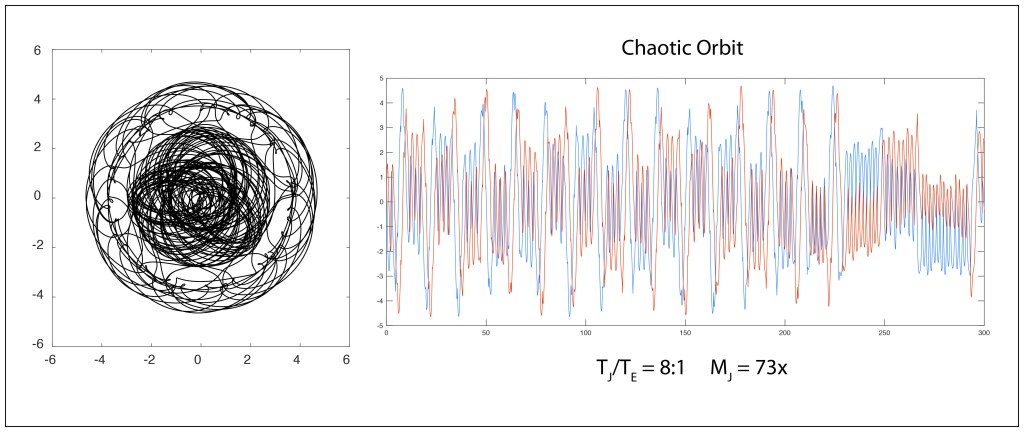
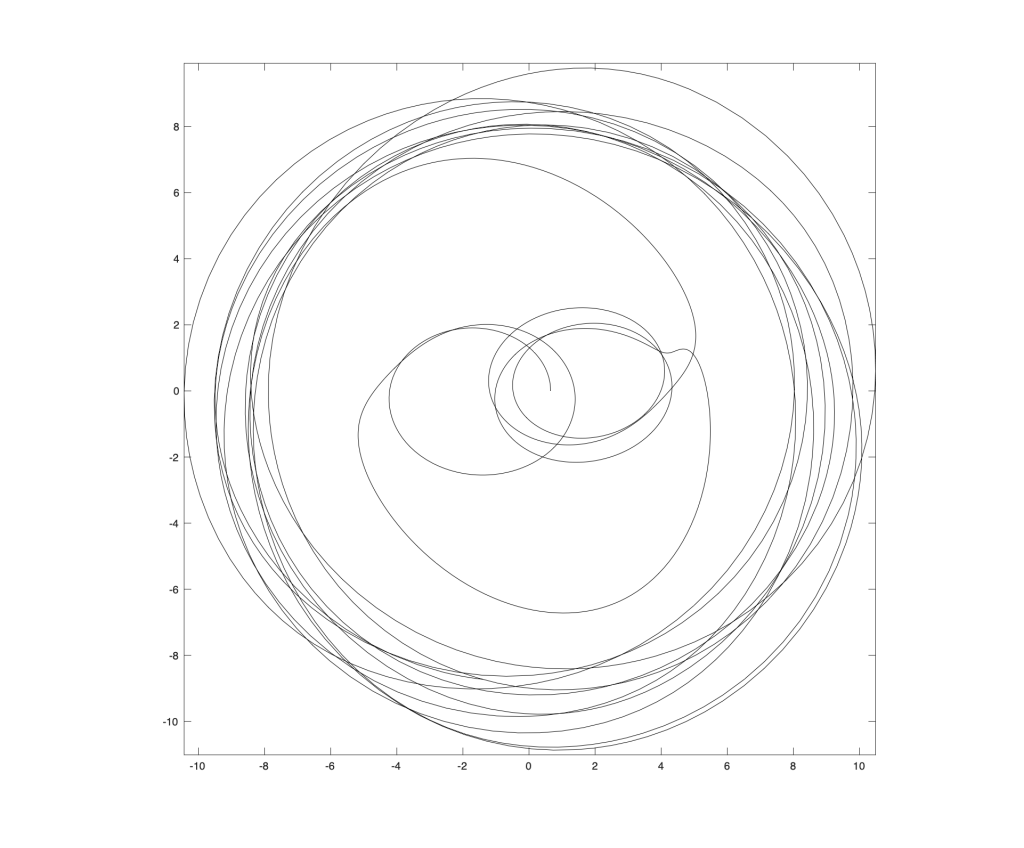
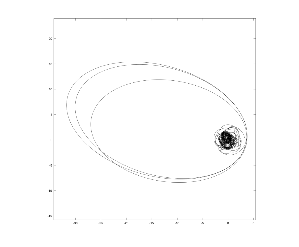
The closest habitable Earth-like exoplanet is Proxima Centauri b, orbiting the red dwarf star Proxima Centauri that is about 4.2 lightyears away from Earth. The planet has a short orbital period of only about 11 Earth days, but the dimness of the red dwarf puts the planet in what may be a habitable zone where water is in liquid form. Its official discovery date was August 24, 2016 by the European Southern Observatory in the Atacama Desert of Chile using the Doppler method. The Alpha Centauri system is a three-star system, and even before the discovery of the planet, this nearest star system to Earth was the inspiration for the Hugo-Award winning sci-fi trilogy The Three Body Problem by Chinese author Liu Cixin, originally published in 2008.

It may seem like a coincidence that the closest Earth-like planet to Earth is in the closest star system to Earth, but it says something about how common such exoplanets may be in our galaxy.

Artist’s rendition of Proxima Centauri b. From WikiCommons.

Breakthrough Starshot

There are already plans to send centimeter-sized spacecraft to Alpha Centauri. One such project that has received a lot of press is Breakthrough Starshot, a project of the Breakthrough Initiatives. Breakthrough Starshot would send around 1000 centimeter-sized camera-carrying laser-fitted spacecraft with 5-meter-diameter solar sails propelled by a large array of high-power lasers. The reason there are so many of these tine spacecraft is because of the collisions that are expected to take place with interstellar dust during the voyage. It is possible that only a few dozen of the craft will finally make it to Alpha Centauri intact.

Relative locations of the stars of the Alpha Centauri system. From ScienceNews.

As these spacecraft fly by the Alpha Centauri system, possibly within one hundred million miles of Proxima Centauri b, their tiny HR digital cameras will take pictures of the planet’s surface with enough resolution to see surface features. The on-board lasers will then transmit the pictures back to Earth. The travel time to the planet is expected to be 20 or 30 years, plus the four years for the laser information to make it back to Earth. Therefore, it would take a quarter century after launch to find out if Proxima Centauri b is habitable or not. The biggest question is whether it has an atmosphere. The red dwarf it orbits sends out catastrophic electromagnetic bursts that could strip the planet of its atmosphere thus preventing any chance for life to evolve or even to be sustained there if introduced.

There are multiple projects under consideration for travel to the Alpha Centauri systems. Even NASA has a tentative mission plan called the 2069 Mission (100 year anniversary of the Moon landing). This would entail a single spacecraft with a much larger solar sail than the small starshot units. Some of the mission plans proposed star-drive technology, such as nuclear propulsion systems, rather than light sails. Some of these designs could sustain a 1-g acceleration throughout the entire mission. It is intriguing to do the math on what such a mission could look like, in terms of travel time. Could we get an unmanned probe to Alpha Centauri in a matter of years? Let’s find out.

Special Relativity of Acceleration

The most surprising aspect of deriving the properties of relativistic acceleration using special relativity is that it works at all. We were all taught as young physicists that special relativity deals with inertial frames in constant motion. So the idea of frames that are accelerating might first seem to be outside the scope of special relativity. But one of Einstein’s key insights, as he sought to extend special relativity towards a more general theory, was that one can define a series of instantaneously inertial co-moving frames relative to an accelerating body. In other words, at any instant in time, the accelerating frame has an inertial co-moving frame. Once this is defined, one can construct invariants, just as in usual special relativity. And these invariants unlock the full mathematical structure of accelerating objects within the scope of special relativity.

For instance, the four-velocity and the four-acceleration in a co-moving frame for an object accelerating at g are given by

The object is momentarily stationary in the co-moving frame, which is why the four-velocity has only the zeroth component, and the four-acceleration has simply g for its first component.

Armed with these four-vectors, one constructs the invariants

and

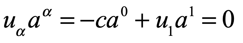
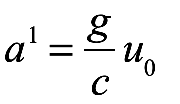
This last equation is solved for the specific co-moving frame as

But the invariant is more general, allowing the expression

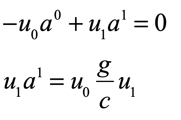
which yields

From these, putting them all together, one obtains the general differential equations for the change in velocity as a set of coupled equations

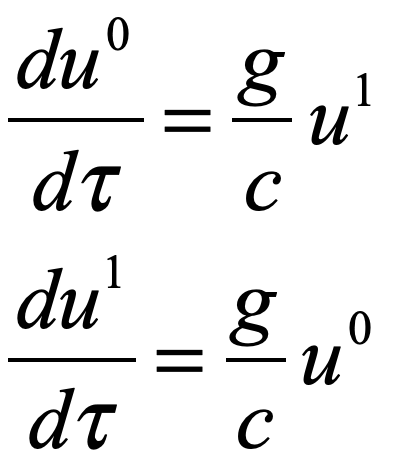
The solution to these equations is

where the unprimed frame is the lab frame (or Earth frame), and the primed frame is the frame of the accelerating object, for instance a starship heading towards Alpha Centauri. These equations allow one to calculate distances, times and speeds as seen in the Earth frame as well as the distances, times and speeds as seen in the starship frame. If the starship is accelerating at some acceleration g’ other than g, then the results are obtained simply by replacing g by g’ in the equations.

Relativistic Flight

It turns out that the acceleration due to gravity on our home planet provides a very convenient (but purely coincidental) correspondence

With a similarly convenient expression

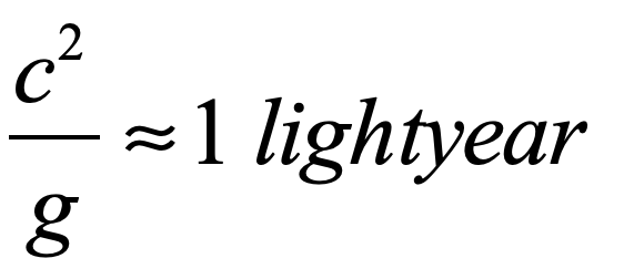
These considerably simplify the math for a starship accelerating at g.

Let’s now consider a starship accelerating by g for the first half of the flight to Alpha Centauri, turning around and decelerating at g for the second half of the flight, so that the starship comes to a stop at its destination. The equations for the times to the half-way point are

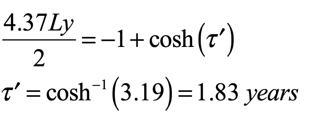
This means at the midpoint that 1.83 years have elapsed on the starship, and about 3 years have elapsed on Earth. The total time to get to Alpha Centauri (and come to a stop) is then simply

It is interesting to look at the speed at the midpoint. This is obtained by

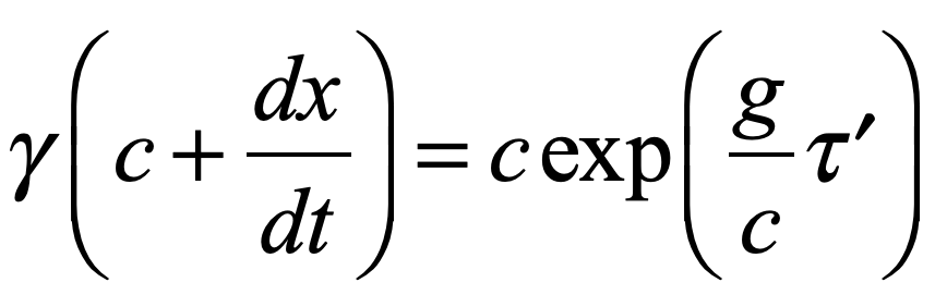
which is solved to give

This amazing result shows that the starship is traveling at 95% of the speed of light at the midpoint when accelerating at the modest value of g for about 3 years. Of course, the engineering challenges for providing such an acceleration for such a long time are currently prohibitive … but who knows? There is a lot of time ahead of us for technology to advance to such a point in the next century or so.

Figure. Time lapsed inside the spacecraft and on Earth for the probe to reach Alpha Centauri as a function of the acceleration of the craft. At 10 g’s, the time elapsed on Earth is a little less than 5 years. However, the signal sent back will take an additional 4.37 years to arrive for a total time of about 9 years.

Matlab alphacentaur.m

% alphacentaur.m
clear
format compact

g0 = 1;
L = 4.37;

for loop = 1:100
    
    g = 0.1*loop*g0;
    
    taup = (1/g)*acosh(g*L/2 + 1);
    tearth = (1/g)*sinh(g*taup);
    
    tauspacecraft(loop) = 2*taup;
    tlab(loop) = 2*tearth;
    
    acc(loop) = g;
    
end

figure(1)
loglog(acc,tauspacecraft,acc,tlab,'LineWidth',2)
legend('Space Craft','Earth Frame','FontSize',18)
xlabel('Acceleration (g)','FontSize',18)
ylabel('Time (years)','FontSize',18)
dum = set(gcf,'Color','White');
H = gca;
H.LineWidth = 2;
H.FontSize = 18;

To Centauri and Beyond

Once we get unmanned probes to Alpha Centauri, it opens the door to star systems beyond. The next closest are Barnards star at 6 Ly away, Luhman 16 at 6.5 Ly, Wise at 7.4 Ly, and Wolf 359 at 7.9 Ly. Several of these are known to have orbiting exoplanets. Ross 128 at 11 Ly and Lyuten at 12.2 Ly have known earth-like planets. There are about 40 known earth-like planets within 40 lightyears from Earth, and likely there are more we haven’t found yet. It is almost inconceivable that none of these would have some kind of life. Finding life beyond our solar system would be a monumental milestone in the history of science. Perhaps that day will come within this century.

By David D. Nolte, March 23, 2022

Life in a Solar System with a Super-sized Jupiter

There are many known super-Jupiters that orbit their stars—they are detected through a slight Doppler wobble they induce on their stars [1]. But what would become of a rocky planet also orbiting those stars as they feel the tug of both the star and the super planet?

This is not of immediate concern for us, because our solar system has had its current configuration of planets for over 4 billion years. But there can be wandering interstellar planets or brown dwarfs that could visit our solar system, like Oumuamua did in 2017, but much bigger and able to scramble the planetary orbits. Such hypothesized astronomical objects have been given the name “Nemesis“, and it warrants thought on what living in an altered solar system might be like.

What would happen to Earth if Jupiter were 50 times bigger? Could we survive?

The Three-Body Problem

The Sun-Earth-Jupiter configuration is a three-body problem that has a long and interesting history, playing a key role in several aspects of modern dynamics [2]. There is no general analytical solution to the three-body problem. To find the behavior of three mutually interacting bodies requires numerical solution. However, there are subsets of the three-body problem that do yield to partial analytical approaches. One of these is called the restricted three-body problem [3]. It consists of two massive bodies plus a third (nearly) massless body that all move in a plane. This restricted problem was first tackled by Euler and later by Poincaré, who discovered the existence of chaos in its solutions.

The geometry of the restricted three-body problem is shown in Fig. 1. In this problem, take mass m₁ = m_S to be the Sun’s mass, m₂ = m_J to be Jupiter’s mass, and the third (small) mass is the Earth.

Fig. 1 The restricted 3-body problem in the plane. The third mass is negligible relative to the first two masses that obey 2-body dynamics.

The equation of motion for the Earth is

where

and the parameter ξ characterizes the strength of the perturbation of the Earth’s orbit around the Sun. The parameters for the Jupiter-Sun system are

with

for the 11.86 year journey of Jupiter around the Sun. Eq. (1) is a four-dimensional non-autonomous flow

The solutions of an Earth orbit are shown in Fig.2. The natural Earth-Sun-Jupiter system has a mass ratio m_J/m_S = 0.001 for Jupiter relative to the Sun mass. Even in this case, Jupiter causes perturbations of the Earth’s orbit by about one percent. If the mass of Jupiter increases, the perturbations would grow larger until around ξ= 0.06 when the perturbations become severe and the orbit grows unstable. The Earth gains energy from the momentum of the Sun-Jupiter system and can reach escape velocity. The simulation for a mass ratio of 0.07 shows the Earth ejected from the Solar System.

Fig.2 Orbit of Earth as a function of the size of a Jupiter-like planet. The natural system has a Jupiter-Earth mass ratio of 0.03. As the size of Jupiter increases, the Earth orbit becomes unstable and can acquire escape velocity to escape from the Solar System. From body3.m. (Reprinted from Ref. [4])

The chances for ejection depends on initial conditions for these simulations, but generally the danger becomes severe when Jupiter is about 50 times larger than it currently is. Otherwise the Earth remains safe from ejection. However, if the Earth is to keep its climate intact, then Jupiter should not be any larger than about 5 times its current size. At the other extreme, for a planet 70 times larger than Jupiter, the Earth may not get ejected at once, but it can take a wild ride through the solar system. A simulation for a 70x Jupiter is shown in Fig. 3. In this case, the Earth is captured for a while as a “moon” of Jupiter in a very tight orbit around the super planet as it orbits the sun before it is set free again to orbit the sun in highly elliptical orbits. Because of the premise of the restricted three-body problem, the Earth has no effect on the orbit of Jupiter.

Fig. 3 Orbit of Earth for T_J = 11.86 years and ξ = 0.069. The radius of Jupiter is R_J = 5.2. Earth is “captured” for a while by Jupiter into a very tight orbit.

Resonance

If Nemesis were to swing by and scramble the solar system, then Jupiter might move closer to the Earth. More ominously, the period of Jupiter’s orbit could come into resonance with the Earth’s period. This occurs when the ratio of orbital periods is a ratio of small integers. Resonance can amplify small perturbations, so perhaps Jupiter would become a danger to Earth. However, the forces exerted by Jupiter on the Earth changes the Earth’s orbit and hence its period, preventing strict resonance to occur, and the Earth is not ejected from the solar system even for initial rational periods or larger planet mass. This is related to the famous KAM theory of resonances by Kolmogorov, Arnold and Moser that tends to protect the Earth from the chaos of the solar system. More often than not in these scenarios, the Earth is either captured by the super Jupiter, or it is thrown into a large orbit that is still bound to the sun. Some examples are given in the following figures.

Fig. 5 Earth orbit for T_J = 12 years and ξ = 0.071. The Earth is thrown into a nearly circular orbit beyond the orbit of Saturn.

Fig. 6 Earth Orbit for T_J = 4 years and ξ = 0.0615. Earth is thrown into an orbit of high ellipticity out to the orbit of Neptune.

Life on a planet in a solar system with two large bodies has been envisioned in dramatic detail in the science fiction novel “Three-Body Problem” by Liu Cixin about the Trisolarians of the closest known exoplanet to Earth–Proxima Centauri b.

By David D. Nolte, Feb. 28, 2022

Matlab Code: body3.m

function body3

clear

chsi0 = 1/1000;     % Earth-moon ratio = 1/317
wj0 = 2*pi/11.86;

wj = 2*pi/8;
chsi = 73*chsi0;    % (11.86,60) (11.86,67.5) (11.86,69) (11.86,70) (4,60) (4,61.5) (8,73) (12,71) 

rj = 5.203*(wj0/wj)^0.6666

rsun = chsi*rj/(1+chsi);
rjup = (1/chsi)*rj/(1+1/chsi);

r0 = 1-rsun;
y0 = [r0 0 0 2*pi/sqrt(r0)];

tspan = [0 300];
options = odeset('RelTol',1e-5,'AbsTol',1e-6);
[t,y] = ode45(@f5,tspan,y0,options);

figure(1)
plot(t,y(:,1),t,y(:,3))

figure(2)
plot(y(:,1),y(:,3),'k')
axis equal
axis([-6 6 -6 6])

RE = sqrt(y(:,1).^2 + y(:,3).^2);
stdRE = std(RE)

%print -dtiff -r800 threebody

    function yd = f5(t,y)
        
        xj = rjup*cos(wj*t);
        yj = rjup*sin(wj*t);
        xs = -rsun*cos(wj*t);
        ys = -rsun*sin(wj*t);
        rj32 = ((y(1) - xj).^2 + (y(3) - yj).^2).^1.5;
        r32 = ((y(1) - xs).^2 + (y(3) - ys).^2).^1.5;

        yp(1) = y(2);
        yp(2) = -4*pi^2*((y(1)-xs)/r32 + chsi*(y(1)-xj)/rj32);
        yp(3) = y(4);
        yp(4) = -4*pi^2*((y(3)-ys)/r32 + chsi*(y(3)-yj)/rj32);
 
        yd = [yp(1);yp(2);yp(3);yp(4)];

    end     % end f5

end

References:

[1] D. D. Nolte, “The Fall and Rise of the Doppler Effect,” Physics Today, vol. 73, no. 3, pp. 31-35, Mar (2020)

[2] J. Barrow-Green, Poincaré and the three body problem. London Mathematical Society, 1997.

[3] M. C. Gutzwiller, “Moon-Earth-Sun: The oldest three-body problem,” Reviews of Modern Physics, vol. 70, no. 2, pp. 589-639, Apr (1998)

[4] D. D. Nolte, Introduction to Modern Dynamics : Chaos, Networks, Space and Time, 1st ed. (Oxford University Press, 2015).

July 19, 2019May 3, 2023 by David D. Nolte

Getting Armstrong, Aldrin and Collins Home from the Moon: Apollo 11 and the Three-Body Problem

Fifty years ago on the 20^th of July at nearly 11 o’clock at night, my brothers and I were peering through the screen door of a very small 1960’s Shasta compact car trailer watching the TV set on the picnic table outside the trailer door. Our family was at a camp ground in southern Michigan and the mosquitos were fierce (hence why we were inside the trailer looking out through the screen). Neil Armstrong was about to be the first human to step foot on the Moon. The image on the TV was a fuzzy black and white, with barely recognizable shapes clouded even more by the dirt and dead bugs on the screen, but it is a memory etched in my mind. I was 10 years old and I was convinced that when I grew up I would visit the Moon myself, because by then Moon travel would be like flying to Europe. It didn’t turn out that way, and fifty years later it’s a struggle to even get back there.

The dangers could have become life-threatening for the crew of Apollo 11. If they miscalculated their trajectory home and had bounced off the Earth’s atmosphere, they would have become a tragic demonstration of the chaos of three-body orbits.

So maybe I won’t get to the Moon, but maybe my grandchildren will. And if they do, I hope they know something about the three-body problem in physics, because getting to and from the Moon isn’t as easy as it sounds. Apollo 11 faced real danger at several critical points on its flight plan, but all went perfectly (except overshooting their landing site and that last boulder field right before Armstrong landed). Some of those dangers became life-threatening for the crew of Apollo 13, and if they had miscalculated their trajectory home and had bounced off the Earth’s atmosphere, they would have become a tragic demonstration of the chaos of three-body orbits. In fact, their lifeless spaceship might have returned to the Moon and back to Earth over and over again, caught in an infinite chaotic web.

The complexities of trajectories in the three-body problem arise because there are too few constants of motion and too many degrees of freedom. To get an intuitive picture of how the trajectory behaves, it is best to start with a problem known as the restricted three-body problem.

The Saturn V Booster, perhaps the pinnacle of “muscle and grit” space exploration.

The Restricted Three-Body Problem

The restricted three-body problem was first considered by Leonhard Euler in 1762 (for a further discussion of the history of the three-body problem, see my Blog from July 5). For the special case of circular orbits of constant angular frequency, the motion of the third mass is described by the Lagrangian

where the potential is time dependent because of the motion of the two larger masses. Lagrange approached the problem by adopting a rotating reference frame in which the two larger masses m₁ and m₂ move along the stationary line defined by their centers. The new angle variable is theta-prime. The Lagrangian in the rotating frame is

where the effective potential is now time independent. The first term in the effective potential is the Coriolis effect and the second is the centrifugal term. The dynamical flow in the plane is four dimensional, and the four-dimensional flow is

where the position vectors are in the center-of-mass frame

relative to the positions of the Earth and Moon (x1 and x2) in the rotating frame in which they are at rest along the x-axis.

A single trajectory solved for this flow is shown in Fig. 1 for a tiny object passing back and forth chaotically between the Earth and the Moon. The object is considered to be massless, or at least so small it does not perturb the Earth-Moon system. The energy of the object was selected to allow it to pass over the potential barrier of the Lagrange-Point L1 between the Earth and the Moon. The object spends most of its time around the Earth, but now and then will get into a transfer orbit that brings it around the Moon. This would have been the fate of Apollo 11 if their last thruster burn had failed.

Fig. 1 The trajectory of a tiny object in the planar three-body problem interacting with a large mass (Earth on the left) and a small mass (Moon on the right). The energy of the trajectory allows it to pass back and forth chaotically between proximity to the Earth and proximity to the Moon. The time-duration of the simulation is approximately one decade. The envelope of the trajectories is called the “Hill region” named after one of the the first US astrophysicists George William Hill (1838-1914) who studied the 3-body problem of the Moon.

Contrast the orbit of Fig. 1 with the simple flight plan of Apollo 11 on the banner figure. The chaotic character of the three-body problem emerges for a “random” initial condition. You can play with different initial conditions in the following Python code to explore the properties of this dynamical problem. Note that in this simulation, the mass of the Moon was chosen about 8 times larger than in nature to exaggerate the effect of the Moon.

Python Code: Hill.py

(Python code on GitHub.)

#!/usr/bin/env python3
# -*- coding: utf-8 -*-
"""
Hill.py
Created on Tue May 28 11:50:24 2019
@author: nolte
D. D. Nolte, Introduction to Modern Dynamics: Chaos, Networks, Space and Time, 2nd ed. (Oxford,2019)
"""

import numpy as np
import matplotlib as mpl
from mpl_toolkits.mplot3d import Axes3D
from scipy import integrate
from matplotlib import pyplot as plt
from matplotlib import cm
import time
import os

plt.close('all')

womega = 1
R = 1
eps = 1e-6

M1 = 1     % Mass of the Earth
M2 = 1/10     % Mass of the Moon
chsi = M2/M1

x1 = -M2*R/(M1+M2)    % Earth location in rotating frame
x2 = x1 + R     % Moon location

def poten(y,c):
    
    rp0 = np.sqrt(y**2 + c**2);
    thetap0 = np.arctan(y/c);
        
    rp1 = np.sqrt(x1**2 + rp0**2 - 2*np.abs(rp0*x1)*np.cos(np.pi-thetap0));
    rp2 = np.sqrt(x2**2 + rp0**2 - 2*np.abs(rp0*x2)*np.cos(thetap0));
    V = -M1/rp1 -M2/rp2 - E;
     
    return [V]

def flow_deriv(x_y_z,tspan):
    x, y, z, w = x_y_z
    
    r1 = np.sqrt(x1**2 + x**2 - 2*np.abs(x*x1)*np.cos(np.pi-z));
    r2 = np.sqrt(x2**2 + x**2 - 2*np.abs(x*x2)*np.cos(z));
        
    yp = np.zeros(shape=(4,))
    yp[0] = y
    yp[1] = -womega**2*R**3*(np.abs(x)-np.abs(x1)*np.cos(np.pi-z))/(r1**3+eps) - womega**2*R**3*chsi*(np.abs(x)-abs(x2)*np.cos(z))/(r2**3+eps) + x*(w-womega)**2
    yp[2] = w
    yp[3] = 2*y*(womega-w)/x - womega**2*R**3*chsi*abs(x2)*np.sin(z)/(x*(r2**3+eps)) + womega**2*R**3*np.abs(x1)*np.sin(np.pi-z)/(x*(r1**3+eps))
    
    return yp
                
r0 = 0.64   % initial radius
v0 = 0.3    % initial radial speed
theta0 = 0   % initial angle
vrfrac = 1   % fraction of speed in radial versus angular directions

rp1 = np.sqrt(x1**2 + r0**2 - 2*np.abs(r0*x1)*np.cos(np.pi-theta0))
rp2 = np.sqrt(x2**2 + r0**2 - 2*np.abs(r0*x2)*np.cos(theta0))
V = -M1/rp1 - M2/rp2
T = 0.5*v0**2
E = T + V

vr = vrfrac*v0
W = (2*T - v0**2)/r0

y0 = [r0, vr, theta0, W]   % This is where you set the initial conditions

tspan = np.linspace(1,2000,20000)

y = integrate.odeint(flow_deriv, y0, tspan)

xx = y[1:20000,0]*np.cos(y[1:20000,2]);
yy = y[1:20000,0]*np.sin(y[1:20000,2]);

plt.figure(1)
lines = plt.plot(xx,yy)
plt.setp(lines, linewidth=0.5)
plt.show()

In the code, set the position and speed of the Apollo command module on lines 56-59 and put in the initial conditions on line 70. The mass of the Moon in nature is 1/81 of the mass of the Earth, which shrinks the L1 “bottleneck” to a much smaller region that you can explore to see what the fate of the Apollo missions could have been.

The Three-Body Problem, Longitude at Sea, and Lagrange’s Points

When Newton developed his theory of universal gravitation, the first problem he tackled was Kepler’s elliptical orbits of the planets around the sun, and he succeeded beyond compare. The second problem he tackled was of more practical importance than the tracks of distant planets, namely the path of the Earth’s own moon, and he was never satisfied.

Newton’s Principia and the Problem of Longitude

Measuring the precise location of the moon at very exact times against the backdrop of the celestial sphere was a method for ships at sea to find their longitude. Yet the moon’s orbit around the Earth is irregular, and Newton recognized that because gravity was universal, every planet exerted a force on each other, and the moon was being tugged upon by the sun as well as by the Earth.

Newton’s attempt with the Moon was his last significant scientific endeavor

In Propositions 65 and 66 of Book 1 of the Principia, Newton applied his new theory to attempt to pin down the moon’s trajectory, but was thwarted by the complexity of the three bodies of the Earth-Moon-Sun system. For instance, the force of the sun on the moon is greater than the force of the Earth on the moon, which raised the question of why the moon continued to circle the Earth rather than being pulled away to the sun. Newton correctly recognized that it was the Earth-moon system that was in orbit around the sun, and hence the sun caused only a perturbation on the Moon’s orbit around the Earth. However, because the Moon’s orbit is approximately elliptical, the Sun’s pull on the Moon is not constant as it swings around in its orbit, and Newton only succeeded in making estimates of the perturbation.

Unsatisfied with his results in the Principia, Newton tried again, beginning in the summer of 1694, but the problem was to too great even for him. In 1702 he published his research, as far as he was able to take it, on the orbital trajectory of the Moon. He could pin down the motion to within 10 arc minutes, but this was not accurate enough for reliable navigation, representing an uncertainty of over 10 kilometers at sea—error enough to run aground at night on unseen shoals. Newton’s attempt with the Moon was his last significant scientific endeavor, and afterwards this great scientist withdrew into administrative activities and other occult interests that consumed his remaining time.

Race for the Moon

The importance of the Moon for navigation was too pressing to ignore, and in the 1740’s a heated competition to be the first to pin down the Moon’s motion developed among three of the leading mathematicians of the day—Leonhard Euler, Jean Le Rond D’Alembert and Alexis Clairaut—who began attacking the lunar problem and each other [1]. Euler in 1736 had published the first textbook on dynamics that used the calculus, and Clairaut had recently returned from Lapland with Maupertuis. D’Alembert, for his part, had placed dynamics on a firm physical foundation with his 1743 textbook. Euler was first to publish with a lunar table in 1746, but there remained problems in his theory that frustrated his attempt at attaining the required level of accuracy.

At nearly the same time Clairaut and D’Alembert revisited Newton’s foiled lunar theory and found additional terms in the perturbation expansion that Newton had neglected. They rushed to beat each other into print, but Clairaut was distracted by a prize competition for the most accurate lunar theory, announced by the Russian Academy of Sciences and refereed by Euler, while D’Alembert ignored the competition, certain that Euler would rule in favor of Clairaut. Clairaut won the prize, but D’Alembert beat him into print.

The rivalry over the moon did not end there. Clairaut continued to improve lunar tables by combining theory and observation, while D’Alembert remained more purely theoretical. A growing animosity between Clairaut and D’Alembert spilled out into the public eye and became a daily topic of conversation in the Paris salons. The difference in their approaches matched the difference in their personalities, with the more flamboyant and pragmatic Clairaut disdaining the purist approach and philosophy of D’Alembert. Clairaut succeeded in publishing improved lunar theory and tables in 1752, followed by Euler in 1753, while D’Alembert’s interests were drawn away towards his activities for Diderot’s Encyclopedia.

The battle over the Moon in the late 1740’s was carried out on the battlefield of perturbation theory. To lowest order, the orbit of the Moon around the Earth is a Keplerian ellipse, and the effect of the Sun, though creating problems for the use of the Moon for navigation, produces only a small modification—a perturbation—of its overall motion. Within a decade or two, the accuracy of perturbation theory calculations, combined with empirical observations, had improved to the point that accurate lunar tables had sufficient accuracy to allow ships to locate their longitude to within a kilometer at sea. The most accurate tables were made by Tobias Mayer, who was awarded posthumously a prize of 3000 pounds by the British Parliament in 1763 for the determination of longitude at sea. Euler received 300 pounds for helping Mayer with his calculations. This was the same prize that was coveted by the famous clockmaker John Harrison and depicted so brilliantly in Dava Sobel’s Longitude (1995).

Lagrange Points

Several years later in 1772 Lagrange discovered an interesting special solution to the planar three-body problem with three massive points each executing an elliptic orbit around the center of mass of the system, but configured such that their positions always coincided with the vertices of an equilateral triangle [2]. He found a more important special solution in the restricted three-body problem that emerged when a massless third body was found to have two stable equilibrium points in the combined gravitational potentials of two massive bodies. These two stable equilibrium points are known as the L4 and L5 Lagrange points. Small objects can orbit these points, and in the Sun-Jupiter system these points are occupied by the Trojan asteroids. Similarly stable Lagrange points exist in the Earth-Moon system where space stations or satellites could be parked.

For the special case of circular orbits of constant angular frequency w, the motion of the third mass is described by the Lagrangian

where the effective potential is now time independent. The first term in the effective potential is the Coriolis effect and the second is the centrifugal term.

Fig. Effective potential for the planar three-body problem and the five Lagrange points where the gradient of the effective potential equals zero. The Lagrange points are displayed on a horizontal cross section of the potential energy shown with equipotential lines. The large circle in the center is the Sun. The smaller circle on the right is a Jupiter-like planet. The points L1, L2 and L3 are each saddle-point equilibria positions and hence unstable. The points L4 and L5 are stable points that can collect small masses that orbit these Lagrange points.

The effective potential is shown in the figure for m₃ = 10m₂. There are five locations where the gradient of the effective potential equals zero. The point L1 is the equilibrium position between the two larger masses. The points L2 and L3 are at positions where the centrifugal force balances the gravitational attraction to the two larger masses. These are also the points that separate local orbits around a single mass from global orbits that orbit the two-body system. The last two Lagrange points at L4 and L5 are at one of the vertices of an equilateral triangle, with the other two vertices at the positions of the larger masses. The first three Lagrange points are saddle points. The last two are at maxima of the effective potential.

L1, lies between Earth and the sun at about 1 million miles from Earth. L1 gets an uninterrupted view of the sun, and is currently occupied by the Solar and Heliospheric Observatory (SOHO) and the Deep Space Climate Observatory. L2 also lies a million miles from Earth, but in the opposite direction of the sun. At this point, with the Earth, moon and sun behind it, a spacecraft can get a clear view of deep space. NASA’s Wilkinson Microwave Anisotropy Probe (WMAP) is currently at this spot measuring the cosmic background radiation left over from the Big Bang. The James Webb Space Telescope will move into this region in 2021.

[1] Gutzwiller, M. C. (1998). “Moon-Earth-Sun: The oldest three-body problem.” Reviews of Modern Physics 70(2): 589-639.

[2] J.L. Lagrange Essai sur le problème des trois corps, 1772, Oeuvres tome 6

Galileo Unbound

Physics and History

Tag / Three-body Problem