Up-side-down Physics: Dynamic Equilibrium and the Inverted Pendulum

In the study of mechanics, the physics student moves through several stages in their education.  The first stage is the Newtonian physics of trajectories and energy and momentum conservation—there are no surprises there.  The second stage takes them to Lagrangians and Hamiltonians—here there are some surprises, especially for rigid body rotations.  Yet even at this stage, most problems have analytical solutions, and most of those solutions are exact.

Any street busker can tell you that an equally good (and more interesting) equilibrium point of a simple pendulum is when the bob is at the top.

It is only at the third stage that physics starts to get really interesting, and when surprising results with important ramifications emerge.  This stage is nonlinear physics.  Most nonlinear problems have no exact analytical solutions, but there are regimes where analytical approximations not only are possible but provide intuitive insights.  One of the best examples of this third stage is the dynamic equilibrium of Kapitsa’s up-side-down pendulum.
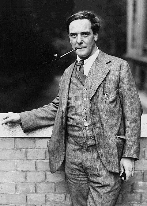
Piotr Kapitsa

Piotr Kapitsa (1894 – 1984) was a Russian physicist who received the Nobel Prize in physics in 1978 for his discovery in 1937 of superfluidity in liquid helium.  (He shared the 1978 prize with Penzias and Wilson who had discovered the cosmic microwave background.)  Superfluidity is a low-temperature hydrodynamic property of superfluids that shares some aspects in common with superconductivity.  Kapitsa published his results in Nature in 1938 in the same issue as a paper by John Allen and Don Misener of Cambridge, but Kapitsa had submitted his paper 19 days before Allen and Misener and so got priority (and the Nobel).

During his career Kapitsa was a leading force in Russian physics, surviving Stalin’s great purge through force of character, and helping to establish the now-famous Moscow Institute of Physics and Technology.  However, surviving Stalin did not always mean surviving with freedom, and around 1950 Kapitsa was under effective house arrest because of his unwillingness to toe the party line.

In his enforced free time, to while away the hours, Kapitsa developed an ingenious analytical approach to the problem of dynamic equilibrium.  His toy example was the driven inverted pendulum. It is surprising how many great works have emerged from the time freed up by house arrest: Galileo finally had time to write his “Two New Sciences”  after his run-in with the Inquisition, and Fresnel was free to develop his theory of diffraction after he ill-advisedly joined a militia to support the Bourbon king during Napoleon’s return. (In our own time, with so many physicists in lock-down and working from home, it will be interesting to see what great theory emerges from the pandemic.)

Stability in the Inverted Driven Pendulum

The only stable static equilibrium of the simple pendulum is when the pendulum bob is at its lowest point.  However, any street busker can tell you that an equally good (and more interesting) equilibrium point is when the bob is at the top.  The caveat is that this “inverted” equilibrium of the pendulum requires active stabilization. 

If the inverted pendulum is a simple physical pendulum, like a meter stick that you balance on the tip of your finger, you know that you need to nudge the stick gently and continuously this way and that with your finger, in response to the tipping stick, to keep it upright.  It’s an easy trick, and almost everyone masters it as a child.  With the human as the drive force, this is an example of a closed-loop control system.  The tipping stick is observed visually by the human, and the finger position is adjusted to compensate for the tip.  On the other hand, one might be interested to find an “open-loop” system that does not require active feedback or even an operator.  In 1908, Andrew Stephenson suggested that induced stability could be achieved by the inverted pendulum if a drive force of sufficiently high frequency were applied [1].  But the proof of the stability remained elusive until Kapitsa followed Stephenson’s suggestion by solving the problem through a separation of time scales [2].

The Method of Separation of Time Scales

The driven inverted pendulum has the dynamical equation

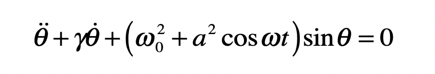
where w0 is the natural angular frequency of small-amplitude oscillations, a is a drive amplitude (with units of frequency) and w is the drive angular frequency that is assumed to be much larger than the natural frequency.  The essential assumption that allows the problem to be separate according to widely separated timescales is that the angular displacement has a slow contribution that changes on the time scale of the natural frequency, and a fast contribution that changes on the time scale of the much higher drive frequency.  The assumed solution then looks like

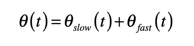
This is inserted into the dynamical equation to yield

where we have used the approximation

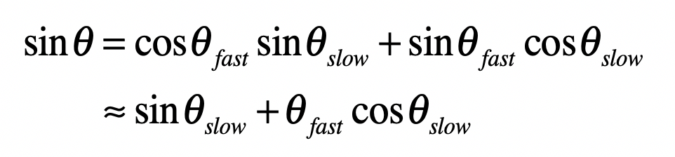
So far this is simple.  The next step is the key step.  It assumes that the dynamical equation should also separate into fast and slow contributions.  But the last term of the sin q expansion has a product of fast and slow components.  The key insight is that a time average can be used to average over the fast contribution.  The separation of the dynamical equation is then

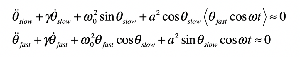
where the time average of the fast variables is only needed on the first line.  The second line is a simple driven harmonic oscillator with a natural frequency that depends on cos qslow and a driving amplitude that depends on sin qslow.  The classic solution to the second line for qfast is

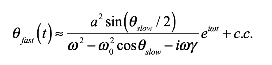
This solution can then be inserted into the first line to yield

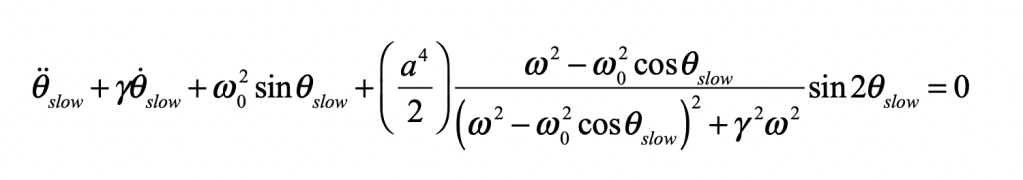
This describes a pendulum under an effective potential (for high drive frequency and no damping)

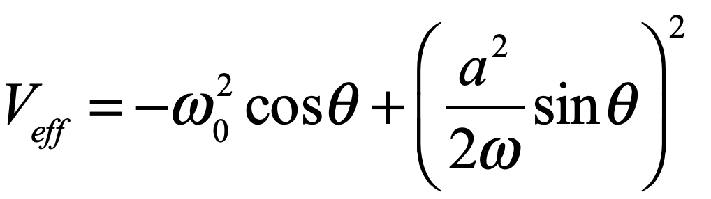
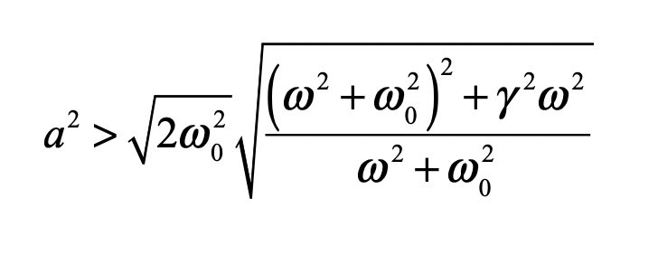
The first term is unstable at the inverted position, but the second term is actually a restoring force.  If the second term is stronger than the first, then a dynamic equilibrium can be achieved. This occurs when the driving amplitude is larger than a threshold value

The effective potential for increasing drive amplitude looks like

Fig. 1 Effective potential as a function of angle and drive amplitude a (in units of w0)

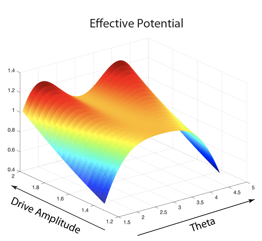
When the drive amplitude is larger than sqrt(2), a slight dip forms in the unstable potential. The dip increases with increasing drive amplitude, as does the oscillation frequency of the effective potential.

Python Program: PenInverted.py

#!/usr/bin/env python3
# -*- coding: utf-8 -*-
"""
PenInverted.py
Created on Friday Sept 11 06:03:32 2020
@author: nolte
D. D. Nolte, Introduction to Modern Dynamics: Chaos, Networks, Space and Time, 2nd ed. (Oxford,2019)
"""

import numpy as np
from scipy import integrate
from matplotlib import pyplot as plt

plt.close('all')

print(' ')
print('PenInverted.py')

F = 133.5          # 30 to 140  (133.5)
delt = 0.000       # 0.000 to 0.01
w = 20          # 20
def flow_deriv(x_y_z,tspan):
    x, y, z = x_y_z
    a = y
    b = -(1 + F*np.cos(z))*np.sin(x) - delt*y
    c = w
    return[a,b,c]
                
T = 2*np.pi/w

x0 = np.pi+0.3
v0 = 0.00
z0 = 0

x_y_z = [x0, v0, z0]

# Solve for the trajectories
t = np.linspace(0, 2000, 200000)
x_t = integrate.odeint(flow_deriv, x_y_z, t)
siztmp = np.shape(x_t)
siz = siztmp[0]

#y1 = np.mod(x_t[:,0]-np.pi,2*np.pi)-np.pi
y1 = x_t[:,0]
y2 = x_t[:,1]
y3 = x_t[:,2]    

plt.figure(1)
lines = plt.plot(t[0:2000],x_t[0:2000,0]/np.pi)
plt.setp(lines, linewidth=0.5)
plt.show()
plt.title('Angular Position')

plt.figure(2)
lines = plt.plot(t[0:1000],y2[0:1000])
plt.setp(lines, linewidth=0.5)
plt.show()
plt.title('Speed')

repnum = 5000
px = np.zeros(shape=(2*repnum,))
xvar = np.zeros(shape=(2*repnum,))
cnt = -1
testwt = np.mod(t,T)-0.5*T;
last = testwt[1]
for loop in range(2,siz-1):
    if (last < 0)and(testwt[loop] > 0):
        cnt = cnt+1
        del1 = -testwt[loop-1]/(testwt[loop] - testwt[loop-1])
        px[cnt] = (y2[loop]-y2[loop-1])*del1 + y2[loop-1]
        xvar[cnt] = (y1[loop]-y1[loop-1])*del1 + y1[loop-1]
        last = testwt[loop]
    else:
        last = testwt[loop]
 
plt.figure(3)
lines = plt.plot(xvar[0:5000],px[0:5000],'ko',ms=1)
plt.show()
plt.title('First Return Map')

plt.figure(4)
lines = plt.plot(x_t[0:1000,0]/np.pi,y2[0:1000])
plt.setp(lines, linewidth=0.5)
plt.show()
plt.title('Phase Space')

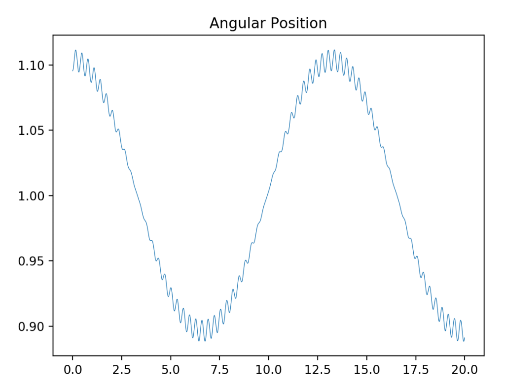
You can play with the parameters of this program to explore the physics of dynamic equilibrium. For instance, if the control parameter is slightly above the threshold (F = 32) at which a dip appears in the effective potential, the slow oscillation has a vary low frequency, as shown in Fig. 2. The high-frequency drive can still be seen superposed on the slow oscillation of the pendulum that is oscillating just like an ordinary pendulum but up-side-down!

Fig. 2 Just above the pitchfork bifurcation the slow oscillation has a low frequency. F = 32, w = 20, w0 = 1

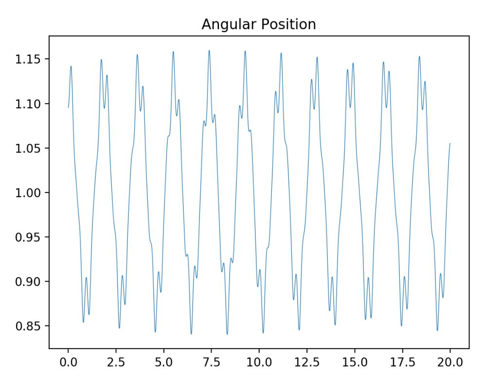
The oscillation frequency is a function of the drive amplitude. This is a classic signature of a nonlinear system: amplitude-frequency coupling. Well above the threshold (F = 100), the frequency of oscillation in the effective potential becomes much larger, as in Fig. 3.

Fig. 3 High above the transition. F = 100, w = 20, w0 = 1

When the drive amplitude is more than four times larger than the threshold value (F > 140), the equilibrium is destroyed, so there is an upper bound to the dynamic stabilization. This happens when the “slow” frequency becomes comparable to the drive frequency and the separation-of-time-scales approach is no longer valid.

You can also play with the damping (delt) to see what effect it has on thresholds and long-term behavior starting at delt = 0.001 and increasing it.

Other Examples of Dynamic Equilibrium

Every physics student learns that there is no stable electrostatic equilibrium. However, if charges are put into motion, then a time-averaged potential can be created that can confine a charged particle. This is the principle of the Paul Ion Trap, named after Wolfgang Paul who was awarded the Nobel Prize in Physics in 1989 for this invention.

One of the most famous examples of dynamic equilibrium are the L4 and L5 Lagrange points. In the Earth-Jupiter system, these are the locations of the Trojan asteroids. These special Lagrange points are maxima (unstable equilibria) in the effective potential of a rotation coordinate system, but the Coriolis force creates a local minimum that traps the asteroids in a dynamically stable equilibrium.

In economics, general equilibrium theory describes how oscillating prices among multiple markets can stabilize economic performance in macroeconomics.

A recent paper in Science magazine used the principle of dynamic equilibrium to levitate a layer of liquid on which toy boats can ride right-side-up and up-side-down. For an interesting video see Upside-down boat (link).

References

[1] Stephenson Andrew (1908). “XX.On induced stability”. Philosophical Magazine. 6. 15: 233–236.

[2] Kapitza P. L. (1951). “Dynamic stability of a pendulum when its point of suspension vibrates”. Soviet Phys. JETP. 21: 588–597.

Links

https://en.wikipedia.org/wiki/Kapitza%27s_pendulum

A detailed derivation of Kapitsa’s approach:https://elmer.unibas.ch/pendulum/upside.htm

The bifurcation threshold for the inverted pendulum is a pitchfork bifurcation https://elmer.unibas.ch/pendulum/bif.htm#pfbif

Getting Armstrong, Aldrin and Collins Home from the Moon: Apollo 11 and the Three-Body Problem

Fifty years ago on the 20th of July at nearly 11 o’clock at night, my brothers and I were peering through the screen door of a very small 1960’s Shasta compact car trailer watching the TV set on the picnic table outside the trailer door.  Our family was at a camp ground in southern Michigan and the mosquitos were fierce (hence why we were inside the trailer looking out through the screen).  Neil Armstrong was about to be the first human to step foot on the Moon.  The image on the TV was a fuzzy black and white, with barely recognizable shapes clouded even more by the dirt and dead bugs on the screen, but it is a memory etched in my mind.  I was 10 years old and I was convinced that when I grew up I would visit the Moon myself, because by then Moon travel would be like flying to Europe.  It didn’t turn out that way, and fifty years later it’s a struggle to even get back there. 

The dangers could have become life-threatening for the crew of Apollo 11. If they miscalculated their trajectory home and had bounced off the Earth’s atmosphere, they would have become a tragic demonstration of the chaos of three-body orbits.

So maybe I won’t get to the Moon, but maybe my grandchildren will.  And if they do, I hope they know something about the three-body problem in physics, because getting to and from the Moon isn’t as easy as it sounds.  Apollo 11 faced real danger at several critical points on its flight plan, but all went perfectly (except overshooting their landing site and that last boulder field right before Armstrong landed). Some of those dangers became life-threatening for the crew of Apollo 13, and if they had miscalculated their trajectory home and had bounced off the Earth’s atmosphere, they would have become a tragic demonstration of the chaos of three-body orbits.  In fact, their lifeless spaceship might have returned to the Moon and back to Earth over and over again, caught in an infinite chaotic web.

The complexities of trajectories in the three-body problem arise because there are too few constants of motion and too many degrees of freedom.  To get an intuitive picture of how the trajectory behaves, it is best to start with a problem known as the restricted three-body problem.

The Saturn V Booster, perhaps the pinnacle of “muscle and grit” space exploration.

The Restricted Three-Body Problem

The restricted three-body problem was first considered by Leonhard Euler in 1762 (for a further discussion of the history of the three-body problem, see my Blog from July 5).  For the special case of circular orbits of constant angular frequency, the motion of the third mass is described by the Lagrangian

where the potential is time dependent because of the motion of the two larger masses.  Lagrange approached the problem by adopting a rotating reference frame in which the two larger masses m1 and m2 move along the stationary line defined by their centers.  The new angle variable is theta-prime.  The Lagrangian in the rotating frame is

where the effective potential is now time independent.  The first term in the effective potential is the Coriolis effect and the second is the centrifugal term.  The dynamical flow in the plane is four dimensional, and the four-dimensional flow is

where the position vectors are in the center-of-mass frame

relative to the positions of the Earth and Moon (x1 and x2) in the rotating frame in which they are at rest along the x-axis.

A single trajectory solved for this flow is shown in Fig. 1 for a tiny object passing back and forth chaotically between the Earth and the Moon. The object is considered to be massless, or at least so small it does not perturb the Earth-Moon system. The energy of the object was selected to allow it to pass over the potential barrier of the Lagrange-Point L1 between the Earth and the Moon. The object spends most of its time around the Earth, but now and then will get into a transfer orbit that brings it around the Moon. This would have been the fate of Apollo 11 if their last thruster burn had failed.

Fig. 1 The trajectory of a tiny object in the planar three-body problem interacting with a large mass (Earth on the left) and a small mass (Moon on the right). The energy of the trajectory allows it to pass back and forth chaotically between proximity to the Earth and proximity to the Moon. The time-duration of the simulation is approximately one decade. The envelope of the trajectories is called the “Hill region” named after one of the the first US astrophysicists George William Hill (1838-1914) who studied the 3-body problem of the Moon.

Contrast the orbit of Fig. 1 with the simple flight plan of Apollo 11 on the banner figure. The chaotic character of the three-body problem emerges for a “random” initial condition. You can play with different initial conditions in the following Python code to explore the properties of this dynamical problem. Note that in this simulation, the mass of the Moon was chosen about 8 times larger than in nature to exaggerate the effect of the Moon.

Python Code: Hill.py

#!/usr/bin/env python3
# -*- coding: utf-8 -*-
"""
Hill.py
Created on Tue May 28 11:50:24 2019
@author: nolte
D. D. Nolte, Introduction to Modern Dynamics: Chaos, Networks, Space and Time, 2nd ed. (Oxford,2019)
"""

import numpy as np
import matplotlib as mpl
from mpl_toolkits.mplot3d import Axes3D
from scipy import integrate
from matplotlib import pyplot as plt
from matplotlib import cm
import time
import os

plt.close('all')

womega = 1
R = 1
eps = 1e-6

M1 = 1     % Mass of the Earth
M2 = 1/10     % Mass of the Moon
chsi = M2/M1

x1 = -M2*R/(M1+M2)    % Earth location in rotating frame
x2 = x1 + R     % Moon location

def poten(y,c):
    
    rp0 = np.sqrt(y**2 + c**2);
    thetap0 = np.arctan(y/c);
        
    rp1 = np.sqrt(x1**2 + rp0**2 - 2*np.abs(rp0*x1)*np.cos(np.pi-thetap0));
    rp2 = np.sqrt(x2**2 + rp0**2 - 2*np.abs(rp0*x2)*np.cos(thetap0));
    V = -M1/rp1 -M2/rp2 - E;
     
    return [V]

def flow_deriv(x_y_z,tspan):
    x, y, z, w = x_y_z
    
    r1 = np.sqrt(x1**2 + x**2 - 2*np.abs(x*x1)*np.cos(np.pi-z));
    r2 = np.sqrt(x2**2 + x**2 - 2*np.abs(x*x2)*np.cos(z));
        
    yp = np.zeros(shape=(4,))
    yp[0] = y
    yp[1] = -womega**2*R**3*(np.abs(x)-np.abs(x1)*np.cos(np.pi-z))/(r1**3+eps) - womega**2*R**3*chsi*(np.abs(x)-abs(x2)*np.cos(z))/(r2**3+eps) + x*(w-womega)**2
    yp[2] = w
    yp[3] = 2*y*(womega-w)/x - womega**2*R**3*chsi*abs(x2)*np.sin(z)/(x*(r2**3+eps)) + womega**2*R**3*np.abs(x1)*np.sin(np.pi-z)/(x*(r1**3+eps))
    
    return yp
                
r0 = 0.64   % initial radius
v0 = 0.3    % initial radial speed
theta0 = 0   % initial angle
vrfrac = 1   % fraction of speed in radial versus angular directions

rp1 = np.sqrt(x1**2 + r0**2 - 2*np.abs(r0*x1)*np.cos(np.pi-theta0))
rp2 = np.sqrt(x2**2 + r0**2 - 2*np.abs(r0*x2)*np.cos(theta0))
V = -M1/rp1 - M2/rp2
T = 0.5*v0**2
E = T + V

vr = vrfrac*v0
W = (2*T - v0**2)/r0

y0 = [r0, vr, theta0, W]   % This is where you set the initial conditions

tspan = np.linspace(1,2000,20000)

y = integrate.odeint(flow_deriv, y0, tspan)

xx = y[1:20000,0]*np.cos(y[1:20000,2]);
yy = y[1:20000,0]*np.sin(y[1:20000,2]);

plt.figure(1)
lines = plt.plot(xx,yy)
plt.setp(lines, linewidth=0.5)
plt.show()

In the code, set the position and speed of the Apollo command module on lines 56-59 and put in the initial conditions on line 70. The mass of the Moon in nature is 1/81 of the mass of the Earth, which shrinks the L1 “bottleneck” to a much smaller region that you can explore to see what the fate of the Apollo missions could have been.

Further Reading

The Three-body Problem, Longitude at Sea, and Lagrange’s Points

Introduction to Modern Dynamics: Chaos, Networks, Space and Time, 2nd Ed. (Oxford University Press, 2019)

The Three-Body Problem, Longitude at Sea, and Lagrange’s Points

When Newton developed his theory of universal gravitation, the first problem he tackled was Kepler’s elliptical orbits of the planets around the sun, and he succeeded beyond compare.  The second problem he tackled was of more practical importance than the tracks of distant planets, namely the path of the Earth’s own moon, and he was never satisfied. 

Newton’s Principia and the Problem of Longitude

Measuring the precise location of the moon at very exact times against the backdrop of the celestial sphere was a method for ships at sea to find their longitude.  Yet the moon’s orbit around the Earth is irregular, and Newton recognized that because gravity was universal, every planet exerted a force on each other, and the moon was being tugged upon by the sun as well as by the Earth.

Newton’s attempt with the Moon was his last significant scientific endeavor

            In Propositions 65 and 66 of Book 1 of the Principia, Newton applied his new theory to attempt to pin down the moon’s trajectory, but was thwarted by the complexity of the three bodies of the Earth-Moon-Sun system.  For instance, the force of the sun on the moon is greater than the force of the Earth on the moon, which raised the question of why the moon continued to circle the Earth rather than being pulled away to the sun. Newton correctly recognized that it was the Earth-moon system that was in orbit around the sun, and hence the sun caused only a perturbation on the Moon’s orbit around the Earth.  However, because the Moon’s orbit is approximately elliptical, the Sun’s pull on the Moon is not constant as it swings around in its orbit, and Newton only succeeded in making estimates of the perturbation. 

            Unsatisfied with his results in the Principia, Newton tried again, beginning in the summer of 1694, but the problem was to too great even for him.  In 1702 he published his research, as far as he was able to take it, on the orbital trajectory of the Moon.  He could pin down the motion to within 10 arc minutes, but this was not accurate enough for reliable navigation, representing an uncertainty of over 10 kilometers at sea—error enough to run aground at night on unseen shoals.  Newton’s attempt with the Moon was his last significant scientific endeavor, and afterwards this great scientist withdrew into administrative activities and other occult interests that consumed his remaining time.

Race for the Moon

            The importance of the Moon for navigation was too pressing to ignore, and in the 1740’s a heated competition to be the first to pin down the Moon’s motion developed among three of the leading mathematicians of the day—Leonhard Euler, Jean Le Rond D’Alembert and Alexis Clairaut—who began attacking the lunar problem and each other [1].  Euler in 1736 had published the first textbook on dynamics that used the calculus, and Clairaut had recently returned from Lapland with Maupertuis.  D’Alembert, for his part, had placed dynamics on a firm physical foundation with his 1743 textbook.  Euler was first to publish with a lunar table in 1746, but there remained problems in his theory that frustrated his attempt at attaining the required level of accuracy.  

            At nearly the same time Clairaut and D’Alembert revisited Newton’s foiled lunar theory and found additional terms in the perturbation expansion that Newton had neglected.  They rushed to beat each other into print, but Clairaut was distracted by a prize competition for the most accurate lunar theory, announced by the Russian Academy of Sciences and refereed by Euler, while D’Alembert ignored the competition, certain that Euler would rule in favor of Clairaut.  Clairaut won the prize, but D’Alembert beat him into print. 

            The rivalry over the moon did not end there. Clairaut continued to improve lunar tables by combining theory and observation, while D’Alembert remained more purely theoretical.  A growing animosity between Clairaut and D’Alembert spilled out into the public eye and became a daily topic of conversation in the Paris salons.  The difference in their approaches matched the difference in their personalities, with the more flamboyant and pragmatic Clairaut disdaining the purist approach and philosophy of D’Alembert.  Clairaut succeeded in publishing improved lunar theory and tables in 1752, followed by Euler in 1753, while D’Alembert’s interests were drawn away towards his activities for Diderot’s Encyclopedia

            The battle over the Moon in the late 1740’s was carried out on the battlefield of perturbation theory.  To lowest order, the orbit of the Moon around the Earth is a Keplerian ellipse, and the effect of the Sun, though creating problems for the use of the Moon for navigation, produces only a small modification—a perturbation—of its overall motion.  Within a decade or two, the accuracy of perturbation theory calculations, combined with empirical observations, had improved to the point that accurate lunar tables had sufficient accuracy to allow ships to locate their longitude to within a kilometer at sea.  The most accurate tables were made by Tobias Mayer, who was awarded posthumously a prize of 3000 pounds by the British Parliament in 1763 for the determination of longitude at sea. Euler received 300 pounds for helping Mayer with his calculations.  This was the same prize that was coveted by the famous clockmaker John Harrison and depicted so brilliantly in Dava Sobel’s Longitude (1995).

Lagrange Points

            Several years later in 1772 Lagrange discovered an interesting special solution to the planar three-body problem with three massive points each executing an elliptic orbit around the center of mass of the system, but configured such that their positions always coincided with the vertices of an equilateral triangle [2].  He found a more important special solution in the restricted three-body problem that emerged when a massless third body was found to have two stable equilibrium points in the combined gravitational potentials of two massive bodies.  These two stable equilibrium points  are known as the L4 and L5 Lagrange points.  Small objects can orbit these points, and in the Sun-Jupiter system these points are occupied by the Trojan asteroids.  Similarly stable Lagrange points exist in the Earth-Moon system where space stations or satellites could be parked. 

For the special case of circular orbits of constant angular frequency w, the motion of the third mass is described by the Lagrangian

where the potential is time dependent because of the motion of the two larger masses.  Lagrange approached the problem by adopting a rotating reference frame in which the two larger masses m1 and m2 move along the stationary line defined by their centers. The Lagrangian in the rotating frame is

where the effective potential is now time independent.  The first term in the effective potential is the Coriolis effect and the second is the centrifugal term.

Fig. Effective potential for the planar three-body problem and the five Lagrange points where the gradient of the effective potential equals zero. The Lagrange points are displayed on a horizontal cross section of the potential energy shown with equipotential lines. The large circle in the center is the Sun. The smaller circle on the right is a Jupiter-like planet. The points L1, L2 and L3 are each saddle-point equilibria positions and hence unstable. The points L4 and L5 are stable points that can collect small masses that orbit these Lagrange points.

            The effective potential is shown in the figure for m3 = 10m2.  There are five locations where the gradient of the effective potential equals zero.  The point L1 is the equilibrium position between the two larger masses.  The points L2 and L3 are at positions where the centrifugal force balances the gravitational attraction to the two larger masses.  These are also the points that separate local orbits around a single mass from global orbits that orbit the two-body system. The last two Lagrange points at L4 and L5 are at one of the vertices of an equilateral triangle, with the other two vertices at the positions of the larger masses. The first three Lagrange points are saddle points.  The last two are at maxima of the effective potential.

L1, lies between Earth and the sun at about 1 million miles from Earth. L1 gets an uninterrupted view of the sun, and is currently occupied by the Solar and Heliospheric Observatory (SOHO) and the Deep Space Climate Observatory. L2 also lies a million miles from Earth, but in the opposite direction of the sun. At this point, with the Earth, moon and sun behind it, a spacecraft can get a clear view of deep space. NASA’s Wilkinson Microwave Anisotropy Probe (WMAP) is currently at this spot measuring the cosmic background radiation left over from the Big Bang. The James Webb Space Telescope will move into this region in 2021.


[1] Gutzwiller, M. C. (1998). “Moon-Earth-Sun: The oldest three-body problem.” Reviews of Modern Physics 70(2): 589-639.

[2] J.L. Lagrange Essai sur le problème des trois corps, 1772, Oeuvres tome 6