
Fifty years ago on the 20th of July at nearly 11 o’clock at night, my brothers and I were peering through the screen door of a very small 1960’s Shasta compact car trailer watching the TV set on the picnic table outside the trailer door. Our family was at a camp ground in southern Michigan and the mosquitos were fierce (hence why we were inside the trailer looking out through the screen). Neil Armstrong was about to be the first human to step foot on the Moon. The image on the TV was a fuzzy black and white, with barely recognizable shapes clouded even more by the dirt and dead bugs on the screen, but it is a memory etched in my mind. I was 10 years old and I was convinced that when I grew up I would visit the Moon myself, because by then Moon travel would be like flying to Europe. It didn’t turn out that way, and fifty years later it’s a struggle to even get back there.
The dangers could have become life-threatening for the crew of Apollo 11. If they miscalculated their trajectory home and had bounced off the Earth’s atmosphere, they would have become a tragic demonstration of the chaos of three-body orbits.
So maybe I won’t get to the Moon, but maybe my grandchildren will. And if they do, I hope they know something about the three-body problem in physics, because getting to and from the Moon isn’t as easy as it sounds. Apollo 11 faced real danger at several critical points on its flight plan, but all went perfectly (except overshooting their landing site and that last boulder field right before Armstrong landed). Some of those dangers became life-threatening for the crew of Apollo 13, and if they had miscalculated their trajectory home and had bounced off the Earth’s atmosphere, they would have become a tragic demonstration of the chaos of three-body orbits. In fact, their lifeless spaceship might have returned to the Moon and back to Earth over and over again, caught in an infinite chaotic web.
The complexities of trajectories in the three-body problem arise because there are too few constants of motion and too many degrees of freedom. To get an intuitive picture of how the trajectory behaves, it is best to start with a problem known as the restricted three-body problem.
The Restricted Three-Body Problem
The restricted three-body problem was first considered by Leonhard Euler in 1762 (for a further discussion of the history of the three-body problem, see my Blog from July 5). For the special case of circular orbits of constant angular frequency, the motion of the third mass is described by the Lagrangian
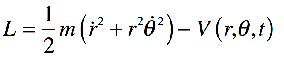
where the potential is time dependent because of the motion of the two larger masses. Lagrange approached the problem by adopting a rotating reference frame in which the two larger masses m1 and m2 move along the stationary line defined by their centers. The new angle variable is theta-prime. The Lagrangian in the rotating frame is
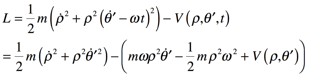
where the effective potential is now time independent. The first term in the effective potential is the Coriolis effect and the second is the centrifugal term. The dynamical flow in the plane is four dimensional, and the four-dimensional flow is
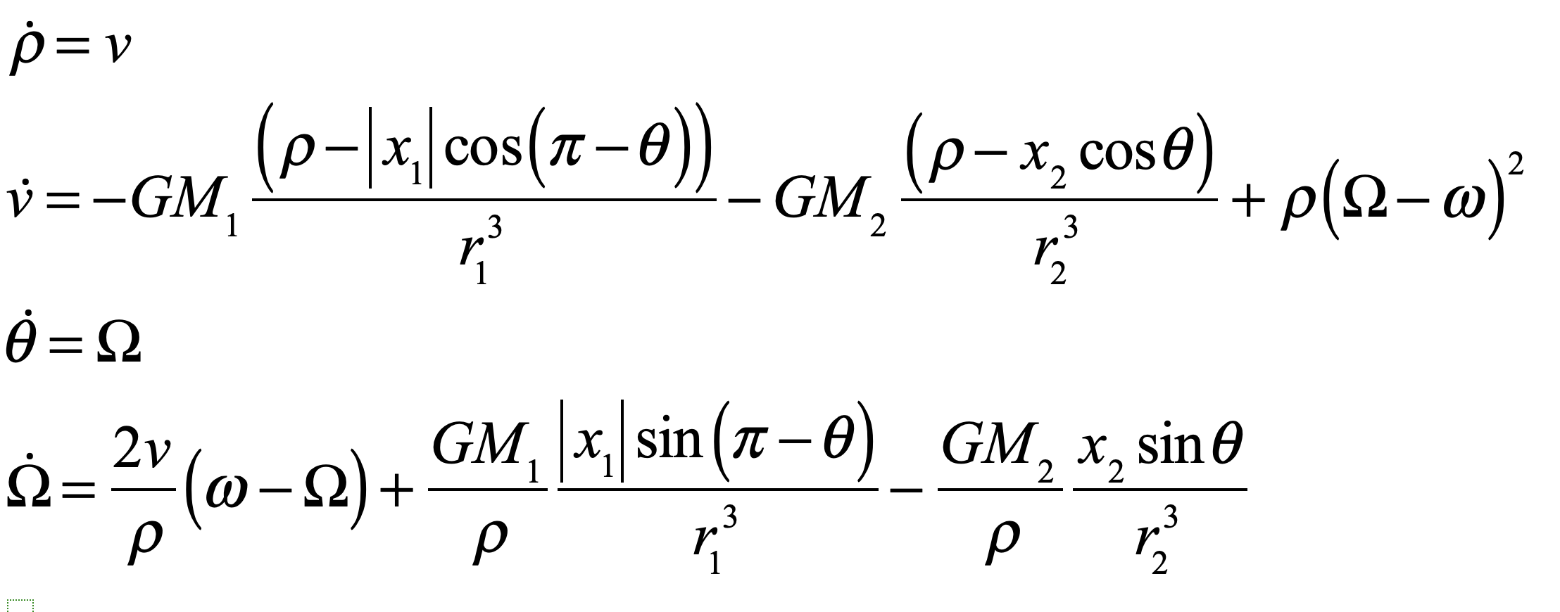
where the position vectors are in the center-of-mass frame
relative to the positions of the Earth and Moon (x1 and x2) in the rotating frame in which they are at rest along the x-axis.
A single trajectory solved for this flow is shown in Fig. 1 for a tiny object passing back and forth chaotically between the Earth and the Moon. The object is considered to be massless, or at least so small it does not perturb the Earth-Moon system. The energy of the object was selected to allow it to pass over the potential barrier of the Lagrange-Point L1 between the Earth and the Moon. The object spends most of its time around the Earth, but now and then will get into a transfer orbit that brings it around the Moon. This would have been the fate of Apollo 11 if their last thruster burn had failed.
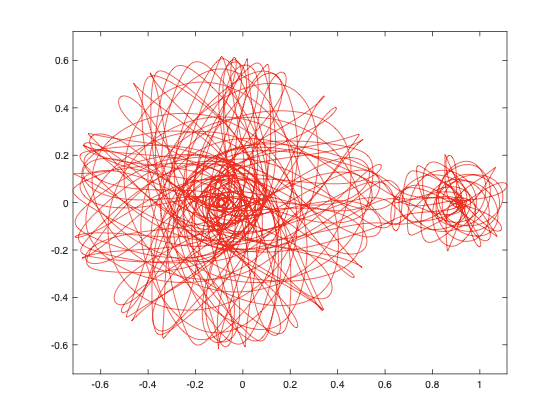
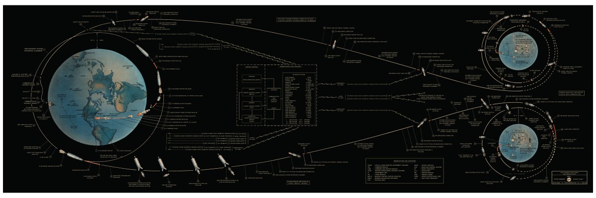
Contrast the orbit of Fig. 1 with the simple flight plan of Apollo 11 on the banner figure. The chaotic character of the three-body problem emerges for a “random” initial condition. You can play with different initial conditions in the following Python code to explore the properties of this dynamical problem. Note that in this simulation, the mass of the Moon was chosen about 8 times larger than in nature to exaggerate the effect of the Moon.
Python Code: Hill.py
(Python code on GitHub.)
#!/usr/bin/env python3
# -*- coding: utf-8 -*-
"""
Hill.py
Created on Tue May 28 11:50:24 2019
@author: nolte
D. D. Nolte, Introduction to Modern Dynamics: Chaos, Networks, Space and Time, 2nd ed. (Oxford,2019)
"""

import numpy as np
import matplotlib as mpl
from mpl_toolkits.mplot3d import Axes3D
from scipy import integrate
from matplotlib import pyplot as plt
from matplotlib import cm
import time
import os

plt.close('all')

womega = 1
R = 1
eps = 1e-6

M1 = 1     % Mass of the Earth
M2 = 1/10     % Mass of the Moon
chsi = M2/M1

x1 = -M2*R/(M1+M2)    % Earth location in rotating frame
x2 = x1 + R     % Moon location

def poten(y,c):

    rp0 = np.sqrt(y**2 + c**2);
    thetap0 = np.arctan(y/c);

    rp1 = np.sqrt(x1**2 + rp0**2 - 2*np.abs(rp0*x1)*np.cos(np.pi-thetap0));
    rp2 = np.sqrt(x2**2 + rp0**2 - 2*np.abs(rp0*x2)*np.cos(thetap0));
    V = -M1/rp1 -M2/rp2 - E;

    return [V]

def flow_deriv(x_y_z,tspan):
    x, y, z, w = x_y_z

    r1 = np.sqrt(x1**2 + x**2 - 2*np.abs(x*x1)*np.cos(np.pi-z));
    r2 = np.sqrt(x2**2 + x**2 - 2*np.abs(x*x2)*np.cos(z));

    yp = np.zeros(shape=(4,))
    yp[0] = y
    yp[1] = -womega**2*R**3*(np.abs(x)-np.abs(x1)*np.cos(np.pi-z))/(r1**3+eps) - womega**2*R**3*chsi*(np.abs(x)-abs(x2)*np.cos(z))/(r2**3+eps) + x*(w-womega)**2
    yp[2] = w
    yp[3] = 2*y*(womega-w)/x - womega**2*R**3*chsi*abs(x2)*np.sin(z)/(x*(r2**3+eps)) + womega**2*R**3*np.abs(x1)*np.sin(np.pi-z)/(x*(r1**3+eps))

    return yp

r0 = 0.64   % initial radius
v0 = 0.3    % initial radial speed
theta0 = 0   % initial angle
vrfrac = 1   % fraction of speed in radial versus angular directions

rp1 = np.sqrt(x1**2 + r0**2 - 2*np.abs(r0*x1)*np.cos(np.pi-theta0))
rp2 = np.sqrt(x2**2 + r0**2 - 2*np.abs(r0*x2)*np.cos(theta0))
V = -M1/rp1 - M2/rp2
T = 0.5*v0**2
E = T + V

vr = vrfrac*v0
W = (2*T - v0**2)/r0

y0 = [r0, vr, theta0, W]   % This is where you set the initial conditions

tspan = np.linspace(1,2000,20000)

y = integrate.odeint(flow_deriv, y0, tspan)

xx = y[1:20000,0]*np.cos(y[1:20000,2]);
yy = y[1:20000,0]*np.sin(y[1:20000,2]);

plt.figure(1)
lines = plt.plot(xx,yy)
plt.setp(lines, linewidth=0.5)
plt.show()
In the code, set the position and speed of the Apollo command module on lines 56-59 and put in the initial conditions on line 70. The mass of the Moon in nature is 1/81 of the mass of the Earth, which shrinks the L1 “bottleneck” to a much smaller region that you can explore to see what the fate of the Apollo missions could have been.
Further Reading
The Three-body Problem, Longitude at Sea, and Lagrange’s Points
