An excerpt from the upcoming book “Interference: The History of Optical Interferometry and the Scientists who Tamed Light” describes how a handful of 19th-century scientists laid the groundwork for one of the key tools of modern optics. Published in Optics and Photonics News, March 2023.
François Arago rose to the highest levels of French science and politics. Along the way, he met Augustin Fresnel and, together, they changed the course of optical science.
In one interpretation of quantum physics, when you snap your fingers, the trajectory you are riding through reality fragments into a cascade of alternative universes—one for each possible quantum outcome among all the different quantum states composing the molecules of your fingers.
This is the Many-Worlds Interpretation (MWI) of quantum physics first proposed rigorously by Hugh Everett in his doctoral thesis in 1957 under the supervision of John Wheeler at Princeton University. Everett had been drawn to this interpretation when he found inconsistencies between quantum physics and gravitation—topics which were supposed to have been his actual thesis topic. But his side-trip into quantum philosophy turned out to be a one-way trip. The reception of his theory was so hostile, no less than from Copenhagen and Bohr himself, that Everett left physics and spent a career at the Pentagon.
Resurrecting MWI in the Name of Quantum Information
Fast forward by 20 years, after Wheeler had left Princeton for the University of Texas at Austin, and once again a young physicist was struggling to reconcile quantum physics with gravity. Once again the many worlds interpretation of quantum physics seemed the only sane way out of the dilemma, and once again a side-trip became a life-long obsession.
David Deutsch, visiting Wheeler in the early 1980’s, became convinced that the many worlds interpretation of quantum physics held the key to paradoxes in the theory of quantum information (For the full story of Wheeler, Everett and Deutsch, see Ref [1]). He was so convinced, that he began a quest to find a physical system that operated on more information than could be present in one universe at a time. If such a physical system existed, it would be because streams of information from more than one universe were coming together and combining in a way that allowed one of the universes to “borrow” the information from the other.
It took only a year or two before Deutsch found what he was looking for—a simple quantum algorithm that yielded twice as much information as would be possible if there were no parallel universes. This is the now-famous Deutsch algorithm—the first quantum algorithm [2]. At the heart of the Deutsch algorithm is a simple quantum interference. The algorithm did nothing useful—but it convinced Deutsch that two universes were interfering coherently in the measurement process, giving that extra bit of information that should not have been there otherwise. A few years later, the Deutsch-Josza algorithm [2] expanded the argument to interfere an exponentially larger amount of information streams from an exponentially larger number of universes to create a result that was exponentially larger than any classical computer could produce. This marked the beginning of the quest for the quantum computer that is running red-hot today.
Deutsch’s “proof” of the many-worlds interpretation of quantum mechanics is not a mathematical proof but is rather a philosophical proof. It holds no sway over how physicists do the math to make their predictions. The Copenhagen interpretation, with its “spooky” instantaneous wavefunction collapse, works just fine predicting the outcome of quantum algorithms and the exponential quantum advantage of quantum computing. Therefore, the story of David Deutsch and the MWI may seem like a chimera—except for one fact—it inspired him to generate the first quantum algorithm that launched what may be the next revolution in the information revolution of modern society. Inspiration is important in science, because it lets scientists create things that had been impossible before.
But if quantum interference is the heart of quantum computing, then there is one physical system that has the ultimate simplicity that may yet inspire future generations of physicists to invent future impossible things—the quantum beam splitter. Nothing in the study of quantum interference can be simpler than a sliver of dielectric material sending single photons one way or another. Yet the outcome of this simple system challenges the mind and reminds us of why Everett and Deutsch embraced the MWI in the first place.
The Classical Beam Splitter
The so-called “beam splitter” is actually a misnomer. Its name implies that it takes a light beam and splits it into two, as if there is only one input. But every “beam splitter” has two inputs, which is clear by looking at the classical 50/50 beam splitter. The actual action of the optical element is the combination of beams into superpositions in each of the outputs. It is only when one of the input fields is zero, a special case, that the optical element acts as a beam splitter. In general, it is a beam combiner.
Given two input fields, the output fields are superpositions of the inputs
The square-root of two factor ensures that energy is conserved, because optical fluence is the square of the fields. This relation is expressed more succinctly as a matrix input-output relation
The phase factors in these equations ensure that the matrix is unitary
reflecting energy conservation.
The Quantum Beam Splitter
A quantum beam splitter is just a classical beam splitter operating at the level of individual photons. Rather than describing single photons entering or leaving the beam splitter, it is more practical to describe the properties of the fields through single-photon quantum operators
where the unitary matrix is the same as the classical case, but with fields replaced by the famous “a” operators. The photon operators operate on single photon modes. For instance, the two one-photon input cases are
where the creation operators operate on the vacuum state in each of the input modes.
The fundamental combinational properties of the beam splitter are even more evident in the quantum case, because there is no such thing as a single input to a quantum beam splitter. Even if no photons are directed into one of the input ports, that port still receives a “vacuum” input, and this vacuum input contributes to the fluctuations observed in the outputs.
The input-output relations for the quantum beam splitter are
The beam splitter operating on a one-photon input converts the input-mode creation operator into a superposition of out-mode creation operators that generates
The resulting output is entangled: either the single photon exits one port, or it exits the other. In the many worlds interpretation, the photon exits from one port in one universe, and it exits from the other port in a different universe. On the other hand, in the Copenhagen interpretation, the two output ports of the beam splitter are perfectly anti-correlated.
Fig. 1 Quantum Operations of a Beam Splitter. A beam splitter creates a quantum superposition of the input modes. The a-symbols are quantum number operators that create and annihilate photons. A single-photon input produces an entangled output that is a quantum superposition of the photon coming out of one output or the other.
The Hong-Ou-Mandel (HOM) Interferometer
When more than one photon is incident on a beam splitter, the fascinating effects of quantum interference come into play, creating unexpected outputs for simple inputs. For instance, the simplest example is a two photon input where a single photon is present in each input port of the beam splitter. The input state is represented with single creation operators operating on each vacuum state of each input port
creating a single photon in each of the input ports. The beam splitter operates on this input state by converting the input-mode creation operators into out-put mode creation operators to give
The important step in this process is the middle line of the equations: There is perfect destructive interference between the two single-photon operations. Therefore, both photons always exit the beam splitter from the same port—never split. Furthermore, the output is an entangled two-photon state, once more splitting universes.
Fig. 2 The HOM interferometer. A two-photon input on a beam splitter generates an entangled superposition of the two photons exiting the beam splitter always together.
The two-photon interference experiment was performed in 1987 by Chung Ki Hong and Jeff Ou, students of Leonard Mandel at the Optics Institute at the University of Rochester [4], and this two-photon operation of the beam splitter is now called the HOM interferometer. The HOM interferometer has become a center-piece for optical and photonic implementations of quantum information processing and quantum computers.
N-Photons on a Beam Splitter
Of course, any number of photons can be input into a beam splitter. For example, take the N-photon input state
The beam splitter acting on this state produces
The quantity on the right hand side can be re-expressed using the binomial theorem
where the permutations are defined by the binomial coefficient
The output state is given by
which is a “super” entangled state composed of N multi-photon states, involving N different universes.
Coherent States on a Quantum Beam Splitter
Surprisingly, there is a multi-photon input state that generates a non-entangled output—as if the input states were simply classical fields. These are the so-called coherent states, introduced by Glauber and Sudarshan [5, 6]. Coherent states can be described as superpositions of multi-photon states, but when a beam splitter operates on these superpositions, the outputs are simply 50/50 mixtures of the states. For instance, if the input scoherent tates are denoted by α and β, then the output states after the beam splitter are
This output is factorized and hence is NOT entangled. This is one of the many reasons why coherent states in quantum optics are considered the “most classical” of quantum states. In this case, a quantum beam splitter operates on the inputs just as if they were classical fields.
By David D. Nolte, May 8, 2022
Read more in “Interference” (New from Oxford University Press, 2023)
A popular account of the trials and toils of the scientists and engineers who tamed light and used it to probe the universe.
[2] D. Deutsch, “Quantum-theory, the church-turing principle and the universal quantum computer,” Proceedings of the Royal Society of London Series a-Mathematical Physical and Engineering Sciences, vol. 400, no. 1818, pp. 97-117, (1985)
[3] D. Deutsch and R. Jozsa, “Rapid solution of problems by quantum computation,” Proceedings of the Royal Society of London Series a-Mathematical Physical and Engineering Sciences, vol. 439, no. 1907, pp. 553-558, Dec (1992)
[4] C. K. Hong, Z. Y. Ou, and L. Mandel, “Measurement of subpicosecond time intervals between 2 photons by interference,” Physical Review Letters, vol. 59, no. 18, pp. 2044-2046, Nov (1987)
[5] Glauber, R. J. (1963). “Photon Correlations.” Physical Review Letters 10(3): 84.
[6] Sudarshan, E. C. G. (1963). “Equivalence of semiclassical and quantum mechanical descriptions of statistical light beams.” Physical Review Letters 10(7): 277-&.; Mehta, C. L. and E. C. Sudarshan (1965). “Relation between quantum and semiclassical description of optical coherence.” Physical Review 138(1B): B274.
The ability to travel to the stars has been one of mankind’s deepest desires. Ever since we learned that we are just one world in a vast universe of limitless worlds, we have yearned to visit some of those others. Yet nature has thrown up an almost insurmountable barrier to that desire–the speed of light. Only by traveling at or near the speed of light may we venture to far-off worlds, and even then, decades or centuries will pass during the voyage. The vast distances of space keep all the worlds isolated–possibly for the better.
Yet the closest worlds are not so far away that they will always remain out of reach. The very limit of the speed of light provides ways of getting there within human lifetimes. The non-intuitive effects of special relativity come to our rescue, and we may yet travel to the closest exoplanet we know of.
Proxima Centauri b
The closest habitable Earth-like exoplanet is Proxima Centauri b, orbiting the red dwarf star Proxima Centauri that is about 4.2 lightyears away from Earth. The planet has a short orbital period of only about 11 Earth days, but the dimness of the red dwarf puts the planet in what may be a habitable zone where water is in liquid form. Its official discovery date was August 24, 2016 by the European Southern Observatory in the Atacama Desert of Chile using the Doppler method. The Alpha Centauri system is a three-star system, and even before the discovery of the planet, this nearest star system to Earth was the inspiration for the Hugo-Award winning sci-fi trilogy The Three Body Problem by Chinese author Liu Cixin, originally published in 2008.
It may seem like a coincidence that the closest Earth-like planet to Earth is in the closest star system to Earth, but it says something about how common such exoplanets may be in our galaxy.
Artist’s rendition of Proxima Centauri b. From WikiCommons.
Breakthrough Starshot
There are already plans to send centimeter-sized spacecraft to Alpha Centauri. One such project that has received a lot of press is Breakthrough Starshot, a project of the Breakthrough Initiatives. Breakthrough Starshot would send around 1000 centimeter-sized camera-carrying laser-fitted spacecraft with 5-meter-diameter solar sails propelled by a large array of high-power lasers. The reason there are so many of these tine spacecraft is because of the collisions that are expected to take place with interstellar dust during the voyage. It is possible that only a few dozen of the craft will finally make it to Alpha Centauri intact.
Relative locations of the stars of the Alpha Centauri system. From ScienceNews.
As these spacecraft fly by the Alpha Centauri system, possibly within one hundred million miles of Proxima Centauri b, their tiny HR digital cameras will take pictures of the planet’s surface with enough resolution to see surface features. The on-board lasers will then transmit the pictures back to Earth. The travel time to the planet is expected to be 20 or 30 years, plus the four years for the laser information to make it back to Earth. Therefore, it would take a quarter century after launch to find out if Proxima Centauri b is habitable or not. The biggest question is whether it has an atmosphere. The red dwarf it orbits sends out catastrophic electromagnetic bursts that could strip the planet of its atmosphere thus preventing any chance for life to evolve or even to be sustained there if introduced.
There are multiple projects under consideration for travel to the Alpha Centauri systems. Even NASA has a tentative mission plan called the 2069 Mission (100 year anniversary of the Moon landing). This would entail a single spacecraft with a much larger solar sail than the small starshot units. Some of the mission plans proposed star-drive technology, such as nuclear propulsion systems, rather than light sails. Some of these designs could sustain a 1-g acceleration throughout the entire mission. It is intriguing to do the math on what such a mission could look like, in terms of travel time. Could we get an unmanned probe to Alpha Centauri in a matter of years? Let’s find out.
Special Relativity of Acceleration
The most surprising aspect of deriving the properties of relativistic acceleration using special relativity is that it works at all. We were all taught as young physicists that special relativity deals with inertial frames in constant motion. So the idea of frames that are accelerating might first seem to be outside the scope of special relativity. But one of Einstein’s key insights, as he sought to extend special relativity towards a more general theory, was that one can define a series of instantaneously inertial co-moving frames relative to an accelerating body. In other words, at any instant in time, the accelerating frame has an inertial co-moving frame. Once this is defined, one can construct invariants, just as in usual special relativity. And these invariants unlock the full mathematical structure of accelerating objects within the scope of special relativity.
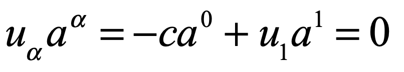
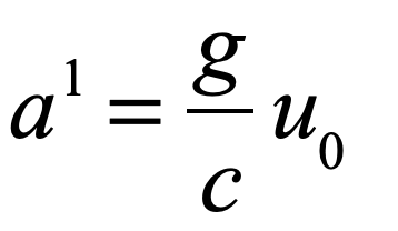
For instance, the four-velocity and the four-acceleration in a co-moving frame for an object accelerating at g are given by
The object is momentarily stationary in the co-moving frame, which is why the four-velocity has only the zeroth component, and the four-acceleration has simply g for its first component.
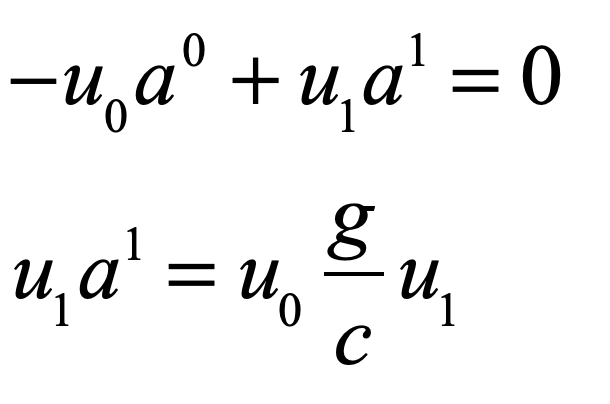
Armed with these four-vectors, one constructs the invariants
and
This last equation is solved for the specific co-moving frame as
But the invariant is more general, allowing the expression
which yields
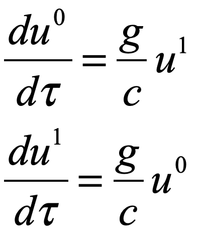
From these, putting them all together, one obtains the general differential equations for the change in velocity as a set of coupled equations
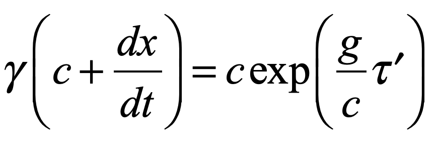
The solution to these equations is
where the unprimed frame is the lab frame (or Earth frame), and the primed frame is the frame of the accelerating object, for instance a starship heading towards Alpha Centauri. These equations allow one to calculate distances, times and speeds as seen in the Earth frame as well as the distances, times and speeds as seen in the starship frame. If the starship is accelerating at some acceleration g’ other than g, then the results are obtained simply by replacing g by g’ in the equations.
Relativistic Flight
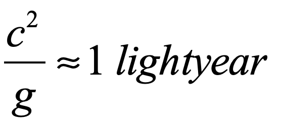
It turns out that the acceleration due to gravity on our home planet provides a very convenient (but purely coincidental) correspondence
With a similarly convenient expression
These considerably simplify the math for a starship accelerating at g.
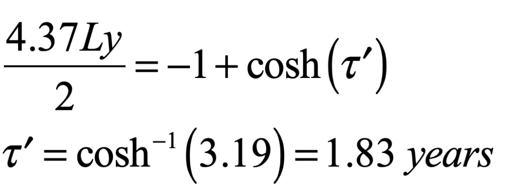
Let’s now consider a starship accelerating by g for the first half of the flight to Alpha Centauri, turning around and decelerating at g for the second half of the flight, so that the starship comes to a stop at its destination. The equations for the times to the half-way point are
This means at the midpoint that 1.83 years have elapsed on the starship, and about 3 years have elapsed on Earth. The total time to get to Alpha Centauri (and come to a stop) is then simply
It is interesting to look at the speed at the midpoint. This is obtained by
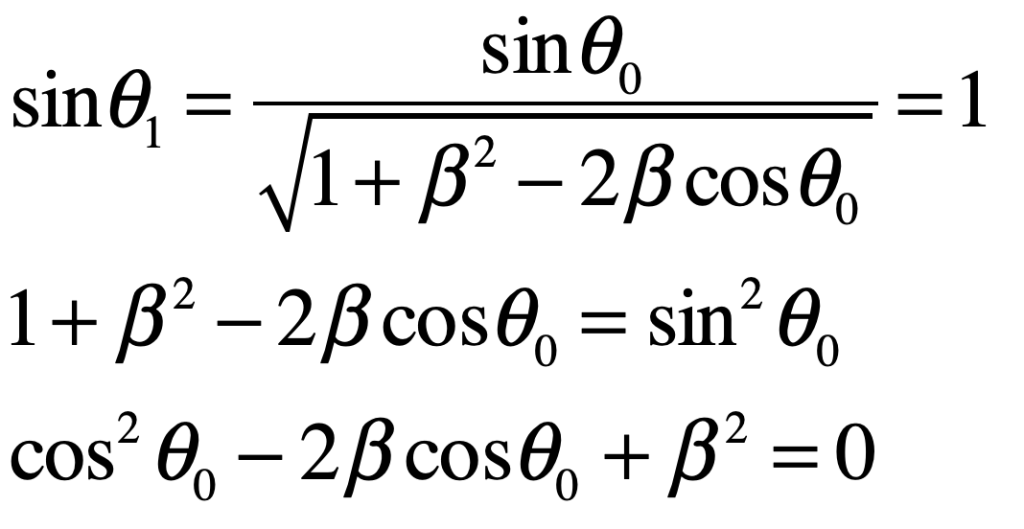
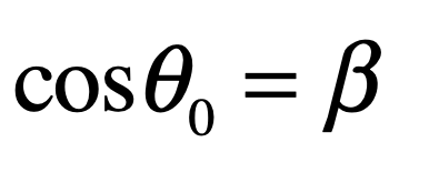
which is solved to give
This amazing result shows that the starship is traveling at 95% of the speed of light at the midpoint when accelerating at the modest value of g for about 3 years. Of course, the engineering challenges for providing such an acceleration for such a long time are currently prohibitive … but who knows? There is a lot of time ahead of us for technology to advance to such a point in the next century or so.
Figure. Time lapsed inside the spacecraft and on Earth for the probe to reach Alpha Centauri as a function of the acceleration of the craft. At 10 g’s, the time elapsed on Earth is a little less than 5 years. However, the signal sent back will take an additional 4.37 years to arrive for a total time of about 9 years.
Matlab alphacentaur.m
% alphacentaur.m
clear
format compact

g0 = 1;
L = 4.37;

for loop = 1:100

    g = 0.1*loop*g0;

    taup = (1/g)*acosh(g*L/2 + 1);
    tearth = (1/g)*sinh(g*taup);

    tauspacecraft(loop) = 2*taup;
    tlab(loop) = 2*tearth;

    acc(loop) = g;

end

figure(1)
loglog(acc,tauspacecraft,acc,tlab,'LineWidth',2)
legend('Space Craft','Earth Frame','FontSize',18)
xlabel('Acceleration (g)','FontSize',18)
ylabel('Time (years)','FontSize',18)
dum = set(gcf,'Color','White');
H = gca;
H.LineWidth = 2;
H.FontSize = 18;
To Centauri and Beyond
Once we get unmanned probes to Alpha Centauri, it opens the door to star systems beyond. The next closest are Barnards star at 6 Ly away, Luhman 16 at 6.5 Ly, Wise at 7.4 Ly, and Wolf 359 at 7.9 Ly. Several of these are known to have orbiting exoplanets. Ross 128 at 11 Ly and Lyuten at 12.2 Ly have known earth-like planets. There are about 40 known earth-like planets within 40 lightyears from Earth, and likely there are more we haven’t found yet. It is almost inconceivable that none of these would have some kind of life. Finding life beyond our solar system would be a monumental milestone in the history of science. Perhaps that day will come within this century.
This Blog Post is a Companion to the undergraduate physics textbook Modern Dynamics: Chaos, Networks, Space and Time, 2nd ed. (Oxford, 2019) introducing Lagrangians and Hamiltonians, chaos theory, complex systems, synchronization, neural networks, econophysics and Special and General Relativity.
If you are a fan of the Doppler effect, then time trials at the Indy 500 Speedway will floor you. Even if you have experienced the fall in pitch of a passing train whistle while stopped in your car at a railroad crossing, or heard the falling whine of a jet passing overhead, I can guarantee that you have never heard anything like an Indy car passing you by at 225 miles an hour.
Indy 500 Time Trials and the Doppler Effect
The Indy 500 time trials are the best way to experience the effect, rather than on race day when there is so much crowd noise and the overlapping sounds of all the cars. During the week before the race, the cars go out on the track, one by one, in time trials to decide the starting order in the pack on race day. Fans are allowed to wander around the entire complex, so you can get right up to the fence at track level on the straight-away. The cars go by only thirty feet away, so they are coming almost straight at you as they approach and straight away from you as they leave. The whine of the car as it approaches is 43% higher than when it is standing still, and it drops to 33% lower than the standing frequency—a ratio almost approaching a factor of two. And they go past so fast, it is almost a step function, going from a steady high note to a steady low note in less than a second. That is the Doppler effect!
But as obvious as the acoustic Doppler effect is to us today, it was far from obvious when it was proposed in 1842 by Christian Doppler at a time when trains, the fastest mode of transport at the time, ran at 20 miles per hour or less. In fact, Doppler’s theory generated so much controversy that the Academy of Sciences of Vienna held a trial in 1853 to decide its merit—and Doppler lost! For the surprising story of Doppler and the fate of his discovery, see my Physics Today article.
From that fraught beginning, the effect has expanded in such importance, that today it is a daily part of our lives. From Doppler weather radar, to speed traps on the highway, to ultrasound images of babies—Doppler is everywhere.
Development of the Doppler-Fizeau Effect
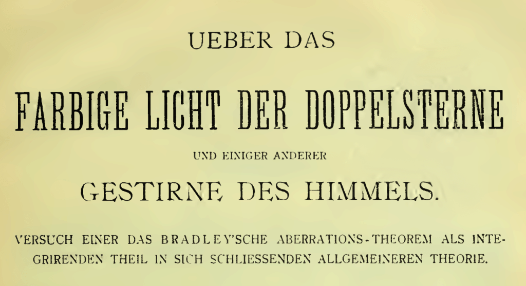
When Doppler proposed the shift in color of the light from stars in 1842 [1], depending on their motion towards or away from us, he may have been inspired by his walk to work every morning, watching the ripples on the surface of the Vltava River in Prague as the water slipped by the bridge piers. The drawings in his early papers look reminiscently like the patterns you see with compressed ripples on the upstream side of the pier and stretched out on the downstream side. Taking this principle to the night sky, Doppler envisioned that binary stars, where one companion was blue and the other was red, was caused by their relative motion. He could not have known at that time that typical binary star speeds were too small to cause this effect, but his principle was far more general, applying to all wave phenomena.
Six years later in 1848 [2], the French physicist Armand Hippolyte Fizeau, soon to be famous for making the first direct measurement of the speed of light, proposed the same principle, unaware of Doppler’s publications in German. As Fizeau was preparing his famous measurement, he originally worked with a spinning mirror (he would ultimately use a toothed wheel instead) and was thinking about what effect the moving mirror might have on the reflected light. He considered the effect of star motion on starlight, just as Doppler had, but realized that it was more likely that the speed of the star would affect the locations of the spectral lines rather than change the color. This is in fact the correct argument, because a Doppler shift on the black-body spectrum of a white or yellow star shifts a bit of the infrared into the visible red portion, while shifting a bit of the ultraviolet out of the visible, so that the overall color of the star remains the same, but Fraunhofer lines would shift in the process. Because of the independent development of the phenomenon by both Doppler and Fizeau, and because Fizeau was a bit clearer in the consequences, the effect is more accurately called the Doppler-Fizeau Effect, and in France sometimes only as the Fizeau Effect. Here in the US, we tend to forget the contributions of Fizeau, and it is all Doppler.
Fig. 1 The title page of Doppler’s 1842 paper [1] proposing the shift in color of stars caused by their motions. (“On the colored light of double stars and a few other stars in the heavens: Study of an integral part of Bradley’s general aberration theory”)
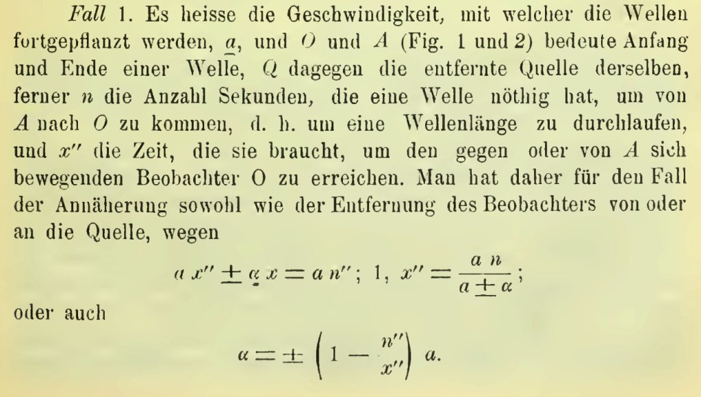
Fig. 2 Doppler used simple proportionality and relative velocities to deduce the first-order change in frequency of waves caused by motion of the source relative to the receiver, or of the receiver relative to the source.
Fig. 3 Doppler’s drawing of what would later be called the Mach cone generating a shock wave. Mach was one of Doppler’s later champions, making dramatic laboratory demonstrations of the acoustic effect, even as skepticism persisted in accepting the phenomenon.
Doppler and Exoplanet Discovery
It is fitting that many of today’s applications of the Doppler effect are in astronomy. His original idea on binary star colors was wrong, but his idea that relative motion changes frequencies was right, and it has become one of the most powerful astrometric techniques in astronomy today. One of its important recent applications was in the discovery of extrasolar planets orbiting distant stars.
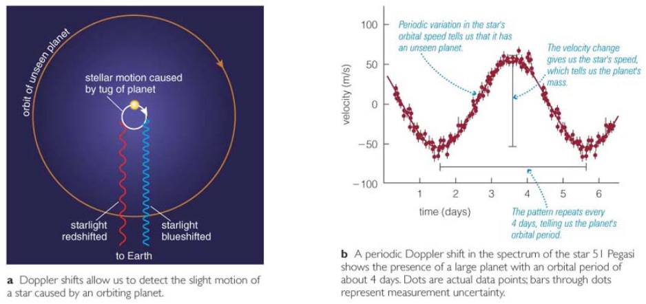
When a large planet like Jupiter orbits a star, the center of mass of the two-body system remains at a constant point, but the individual centers of mass of the planet and the star both orbit the common point. This makes it look like the star has a wobble, first moving towards our viewpoint on Earth, then moving away. Because of this relative motion of the star, the light can appear blueshifted caused by the Doppler effect, then redshifted with a set periodicity. This was observed by Queloz and Mayer in 1995 for the star 51 Pegasi, which represented the first detection of an exoplanet [3]. The duo won the Nobel Prize in 2019 for the discovery.
Fig. 4 A gas giant (like Jupiter) and a star obit a common center of mass causing the star to wobble. The light of the star when viewed at Earth is periodically red- and blue-shifted by the Doppler effect. From Ref.
Doppler and Vera Rubins’ Galaxy Velocity Curves
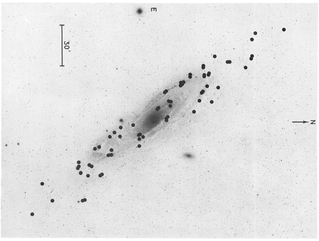
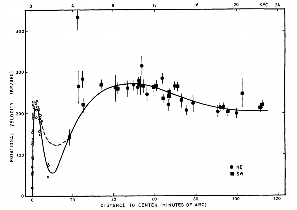
In the late 1960’s and early 1970’s Vera Rubin at the Carnegie Institution of Washington used newly developed spectrographs to use the Doppler effect to study the speeds of ionized hydrogen gas surrounding massive stars in individual galaxies [4]. From simple Newtonian dynamics it is well understood that the speed of stars as a function of distance from the galactic center should increase with increasing distance up to the average radius of the galaxy, and then should decrease at larger distances. This trend in speed as a function of radius is called a rotation curve. As Rubin constructed the rotation curves for many galaxies, the increase of speed with increasing radius at small radii emerged as a clear trend, but the stars farther out in the galaxies were all moving far too fast. In fact, they are moving so fast that they exceeded escape velocity and should have flown off into space long ago. This disturbing pattern was repeated consistently in one rotation curve after another for many galaxies.
Fig. 5 Locations of Doppler shifts of ionized hydrogen measured by Vera Rubin on the Andromeda galaxy. From Ref.
Fig. 6 Vera Rubin’s velocity curve for the Andromeda galaxy. From Ref.
Fig. 7 Measured velocity curves relative to what is expected from the visible mass distribution of the galaxy. From Ref.
A simple fix to the problem of the rotation curves is to assume that there is significant mass present in every galaxy that is not observable either as luminous matter or as interstellar dust. In other words, there is unobserved matter, dark matter, in all galaxies that keeps all their stars gravitationally bound. Estimates of the amount of dark matter needed to fix the velocity curves is about five times as much dark matter as observable matter. In short, 80% of the mass of a galaxy is not normal. It is neither a perturbation nor an artifact, but something fundamental and large. The discovery of the rotation curve anomaly by Rubin using the Doppler effect stands as one of the strongest evidence for the existence of dark matter.
There is so much dark matter in the Universe that it must have a major effect on the overall curvature of space-time according to Einstein’s field equations. One of the best probes of the large-scale structure of the Universe is the afterglow of the Big Bang, known as the cosmic microwave background (CMB).
Doppler and the Big Bang
The Big Bang was astronomically hot, but as the Universe expanded it cooled. About 380,000 years after the Big Bang, the Universe cooled sufficiently that the electron-proton plasma that filled space at that time condensed into hydrogen. Plasma is charged and opaque to photons, while hydrogen is neutral and transparent. Therefore, when the hydrogen condensed, the thermal photons suddenly flew free and have continued unimpeded, continuing to cool. Today the thermal glow has reached about three degrees above absolute zero. Photons in thermal equilibrium with this low temperature have an average wavelength of a few millimeters corresponding to microwave frequencies, which is why the afterglow of the Big Bang got its name: the Cosmic Microwave Background (CMB).
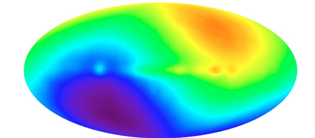
Not surprisingly, the CMB has no preferred reference frame, because every point in space is expanding relative to every other point in space. In other words, space itself is expanding. Yet soon after the CMB was discovered by Arno Penzias and Robert Wilson (for which they were awarded the Nobel Prize in Physics in 1978), an anisotropy was discovered in the background that had a dipole symmetry caused by the Doppler effect as the Solar System moves at 368±2 km/sec relative to the rest frame of the CMB. Our direction is towards galactic longitude 263.85o and latitude 48.25o, or a bit southwest of Virgo. Interestingly, the local group of about 100 galaxies, of which the Milky Way and Andromeda are the largest members, is moving at 627±22 km/sec in the direction of galactic longitude 276o and latitude 30o. Therefore, it seems like we are a bit slack in our speed compared to the rest of the local group. This is in part because we are being pulled towards Andromeda in roughly the opposite direction, but also because of the speed of the solar system in our Galaxy.
Fig. 8 The CMB dipole anisotropy caused by the Doppler effect as the Earth moves at 368 km/sec through the rest frame of the CMB.
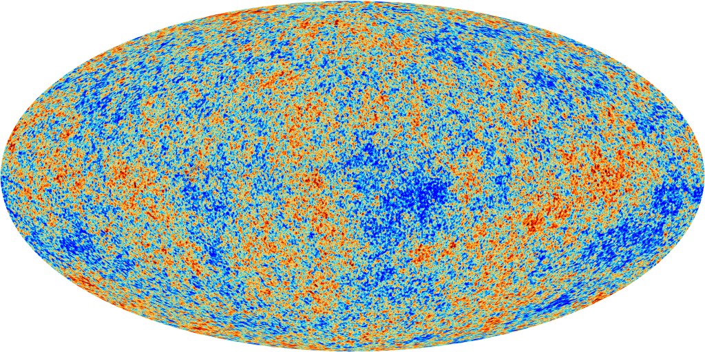
Aside from the dipole anisotropy, the CMB is amazingly uniform when viewed from any direction in space, but not perfectly uniform. At the level of 0.005 percent, there are variations in the temperature depending on the location on the sky. These fluctuations in background temperature are called the CMB anisotropy, and they help interpret current models of the Universe. For instance, the average angular size of the fluctuations is related to the overall curvature of the Universe. This is because, in the early Universe, not all parts of it were in communication with each other. This set an original spatial size to thermal discrepancies. As the Universe continued to expand, the size of the regional variations expanded with it, and the sizes observed today would appear larger or smaller, depending on how the universe is curved. Therefore, to measure the energy density of the Universe, and hence to find its curvature, required measurements of the CMB temperature that were accurate to better than a part in 10,000.
Equivalently, parts of the early universe had greater mass density than others, causing the gravitational infall of matter towards these regions. Then, through the Doppler effect, light emitted (or scattered) by matter moving towards these regions contributes to the anisotropy. They contribute what are known as “Doppler peaks” in the spatial frequency spectrum of the CMB anisotropy.
Fig. 9 The CMB small-scale anisotropy, part of which is contributed by Doppler shifts of matter falling into denser regions in the early universe.
The examples discussed in this blog (exoplanet discovery, galaxy rotation curves, and cosmic background) are just a small sampling of the many ways that the Doppler effect is used in Astronomy. But clearly, Doppler has played a key role in the long history of the universe.
By David D. Nolte, Jan. 23, 2022
References:
[1] C. A. DOPPLER, “Über das farbige Licht der Doppelsterne und einiger anderer Gestirne des Himmels (About the coloured light of the binary stars and some other stars of the heavens),” Proceedings of the Royal Bohemian Society of Sciences, vol. V, no. 2, pp. 465–482, (Reissued 1903) (1842)
[2] H. Fizeau, “Acoustique et optique,” presented at the Société Philomathique de Paris, Paris, 1848.
[3] M. Mayor and D. Queloz, “A JUPITER-MASS COMPANION TO A SOLAR-TYPE STAR,” Nature, vol. 378, no. 6555, pp. 355-359, Nov (1995)
[4] Rubin, Vera; Ford, Jr., W. Kent (1970). “Rotation of the Andromeda Nebula from a Spectroscopic Survey of Emission Regions”. The Astrophysical Journal. 159: 379
M. Tegmark, “Doppler peaks and all that: CMB anisotropies and what they can tell us,” in International School of Physics Enrico Fermi Course 132 on Dark Matter in the Universe, Varenna, Italy, Jul 25-Aug 04 1995, vol. 132, in Proceedings of the International School of Physics Enrico Fermi, 1996, pp. 379-416
Now is exactly the wrong moment to be reviewing the state of photonic quantum computing — the field is moving so rapidly, at just this moment, that everything I say here now will probably be out of date in just a few years. On the other hand, now is exactly the right time to be doing this review, because so much has happened in just the past few years, that it is important to take a moment and look at where this field is today and where it will be going.
At the 20-year anniversary of the publication of my book Mind at Light Speed (Free Press, 2001), this blog is the third in a series reviewing progress in three generations of Machines of Light over the past 20 years (see my previous blogs on the future of the photonic internet and on all-optical computers). This third and final update reviews progress on the third generation of the Machines of Light: the Quantum Optical Generation. Of the three generations, this is the one that is changing the fastest.
Quantum computing is almost here … and it will be at room temperature, using light, in photonic integrated circuits!
Quantum Computing with Linear Optics
Twenty years ago in 2001, Emanuel Knill and Raymond LaFlamme at Los Alamos National Lab, with Gerald Mulburn at the University of Queensland, Australia, published a revolutionary theoretical paper (known as KLM) in Nature on quantum computing with linear optics: “A scheme for efficient quantum computation with linear optics” [1]. Up until that time, it was believed that a quantum computer — if it was going to have the property of a universal Turing machine — needed to have at least some nonlinear interactions among qubits in a quantum gate. For instance, an example of a two-qubit gate is a controlled-NOT, or CNOT, gate shown in Fig. 1 with the Truth Table and the equivalent unitary matrix. It clear that one qubit is controlling the other, telling it what to do.
The quantum CNOT gate gets interesting when the control line has a quantum superposition, then the two outputs become entangled.
Entanglement is a strange process that is unique to quantum systems and has no classical analog. It also has no simple intuitive explanation. By any normal logic, if the control line passes through the gate unaltered, then absolutely nothing interesting should be happening on the Control-Out line. But that’s not the case. The control line going in was a separate state. If some measurement were made on it, either a 1 or 0 would be seen with equal probability. But coming out of the CNOT, the signal has somehow become perfectly correlated with whatever value is on the Signal-Out line. If the Signal-Out is measured, the measurement process collapses the state of the Control-Out to a value equal to the measured signal. The outcome of the control line becomes 100% certain even though nothing was ever done to it! This entanglement generation is one reason the CNOT is often the gate of choice when constructing quantum circuits to perform interesting quantum algorithms.
However, optical implementation of a CNOT is a problem, because light beams and photons really do not like to interact with each other. This is the problem with all-optical classical computers too (see my previous blog). There are ways of getting light to interact with light, for instance inside nonlinear optical materials. And in the case of quantum optics, a single atom in an optical cavity can interact with single photons in ways that can act like a CNOT or related gates. But the efficiencies are very low and the costs to implement it are very high, making it difficult or impossible to scale such systems up into whole networks needed to make a universal quantum computer.
Therefore, when KLM published their idea for quantum computing with linear optics, it caused a shift in the way people were thinking about optical quantum computing. A universal optical quantum computer could be built using just light sources, beam splitters and photon detectors.
The way that KLM gets around the need for a direct nonlinear interaction between two photons is to use postselection. They run a set of photons — signal photons and ancilla (test) photons — through their linear optical system and they detect (i.e., theoretically…the paper is purely a theoretical proposal) the ancilla photons. If these photons are not detected where they are wanted, then that iteration of the computation is thrown out, and it is tried again and again, until the photons end up where they need to be. When the ancilla outcomes are finally what they need to be, this run is selected because the signal state are known to have undergone a known transformation. The signal photons are still unmeasured at this point and are therefore in quantum superpositions that are useful for quantum computation. Postselection uses entanglement and measurement collapse to put the signal photons into desired quantum states. Postselection provides an effective nonlinearity that is induced by the wavefunction collapse of the entangled state. Of course, the down side of this approach is that many iterations are thrown out — the computation becomes non-deterministic.
KLM could get around most of the non-determinism by using more and more ancilla photons, but this has the cost of blowing up the size and cost of the implementation, so their scheme was not imminently practical. But the important point was that it introduced the idea of linear quantum computing. (For this, Milburn and his collaborators have my vote for a future Nobel Prize.) Once that idea was out, others refined it, and improved upon it, and found clever ways to make it more efficient and more scalable. Many of these ideas relied on a technology that was co-evolving with quantum computing — photonic integrated circuits (PICs).
Quantum Photonic Integrated Circuits (QPICs)
Never underestimate the power of silicon. The amount of time and energy and resources that have now been invested in silicon device fabrication is so astronomical that almost nothing in this world can displace it as the dominant technology of the present day and the future. Therefore, when a photon can do something better than an electron, you can guess that eventually that photon will be encased in a silicon chip–on a photonic integrated circuit (PIC).
The dream of integrated optics (the optical analog of integrated electronics) has been around for decades, where waveguides take the place of conducting wires, and interferometers take the place of transistors — all miniaturized and fabricated in the thousands on silicon wafers. The advantages of PICs are obvious, but it has taken a long time to develop. When I was a post-doc at Bell Labs in the late 1980’s, everyone was talking about PICs, but they had terrible fabrication challenges and terrible attenuation losses. Fortunately, these are just technical problems, not limited by any fundamental laws of physics, so time (and an army of researchers) has chipped away at them.
One of the driving forces behind the maturation of PIC technology is photonic fiber optic communications (as discussed in a previous blog). Photons are clear winners when it comes to long-distance communications. In that sense, photonic information technology is a close cousin to silicon — photons are no less likely to be replaced by a future technology than silicon is. Therefore, it made sense to bring the photons onto the silicon chips, tapping into the full array of silicon fab resources so that there could be seamless integration between fiber optics doing the communications and the photonic chips directing the information. Admittedly, photonic chips are not yet all-optical. They still use electronics to control the optical devices on the chip, but this niche for photonics has provided a driving force for advancements in PIC fabrication.
Fig. 2 Schematic of a silicon photonic integrated circuit (PIC). The waveguides can be silica or nitride deposited on the silicon chip. From the Comsol WebSite.
One side-effect of improved PIC fabrication is low light losses. In telecommunications, this loss is not so critical because the systems use OEO regeneration. But less loss is always good, and the PICs can now safeguard almost every photon that comes on chip — exactly what is needed for a quantum PIC. In a quantum photonic circuit, every photon is valuable and informative and needs to be protected. The new PIC fabrication can do this. In addition, light switches for telecom applications are built from integrated interferometers on the chip. It turns out that interferometers at the single-photon level are unitary quantum gates that can be used to build universal photonic quantum computers. So the same technology and control that was used for telecom is just what is needed for photonic quantum computers. In addition, integrated optical cavities on the PICs, which look just like wavelength filters when used for classical optics, are perfect for producing quantum states of light known as squeezed light that turn out to be valuable for certain specialty types of quantum computing.
Therefore, as the concepts of linear optical quantum computing advanced through that last 20 years, the hardware to implement those concepts also advanced, driven by a highly lucrative market segment that provided the resources to tap into the vast miniaturization capabilities of silicon chip fabrication. Very fortuitous!
Room-Temperature Quantum Computers
There are many radically different ways to make a quantum computer. Some are built of superconducting circuits, others are made from semiconductors, or arrays of trapped ions, or nuclear spins on nuclei on atoms in molecules, and of course with photons. Up until about 5 years ago, optical quantum computers seemed like long shots. Perhaps the most advanced technology was the superconducting approach. Superconducting quantum interference devices (SQUIDS) have exquisite sensitivity that makes them robust quantum information devices. But the drawback is the cold temperatures that are needed for them to work. Many of the other approaches likewise need cold temperature–sometimes astronomically cold temperatures that are only a few thousandths of a degree above absolute zero Kelvin.
Cold temperatures and quantum computing seemed a foregone conclusion — you weren’t ever going to separate them — and for good reason. The single greatest threat to quantum information is decoherence — the draining away of the kind of quantum coherence that allows interferences and quantum algorithms to work. In this way, entanglement is a two-edged sword. On the one hand, entanglement provides one of the essential resources for the exponential speed-up of quantum algorithms. But on the other hand, if a qubit “sees” any environmental disturbance, then it becomes entangled with that environment. The entangling of quantum information with the environment causes the coherence to drain away — hence decoherence. Hot environments disturb quantum systems much more than cold environments, so there is a premium for cooling the environment of quantum computers to as low a temperature as they can. Even so, decoherence times can be microseconds to milliseconds under even the best conditions — quantum information dissipates almost as fast as you can make it.
Enter the photon! The bottom line is that photons don’t interact. They are blind to their environment. This is what makes them perfect information carriers down fiber optics. It is also what makes them such good qubits for carrying quantum information. You can prepare a photon in a quantum superposition just by sending it through a lossless polarizing crystal, and then the superposition will last for as long as you can let the photon travel (at the speed of light). Sometimes this means putting the photon into a coil of fiber many kilometers long to store it, but that is OK — a kilometer of coiled fiber in the lab is no bigger than a few tens of centimeters. So the same properties that make photons excellent at carrying information also gives them very small decoherence. And after the KLM schemes began to be developed, the non-interacting properties of photons were no longer a handicap.
In the past 5 years there has been an explosion, as well as an implosion, of quantum photonic computing advances. The implosion is the level of integration which puts more and more optical elements into smaller and smaller footprints on silicon PICs. The explosion is the number of first-of-a-kind demonstrations: the first universal optical quantum computer [2], the first programmable photonic quantum computer [3], and the first (true) quantum computational advantage [4].
All of these “firsts” operate at room temperature. (There is a slight caveat: The photon-number detectors are actually superconducting wire detectors that do need to be cooled. But these can be housed off-chip and off-rack in a separate cooled system that is coupled to the quantum computer by — no surprise — fiber optics.) These are the advantages of photonic quantum computers: hundreds of qubits integrated onto chips, room-temperature operation, long decoherence times, compatibility with telecom light sources and PICs, compatibility with silicon chip fabrication, universal gates using postselection, and more. Despite the head start of some of the other quantum computing systems, photonics looks like it will be overtaking the others within only a few years to become the dominant technology for the future of quantum computing. And part of that future is being helped along by a new kind of quantum algorithm that is perfectly suited to optics.
Fig. 3 Superconducting photon counting detector. From WebSite
A New Kind of Quantum Algorithm: Boson Sampling
In 2011, Scott Aaronson (then at at MIT) published a landmark paper titled “The Computational Complexity of Linear Optics” with his post-doc, Anton Arkhipov [5]. The authors speculated on whether there could be an application of linear optics, not requiring the costly step of post-selection, that was still useful for applications, while simultaneously demonstrating quantum computational advantage. In other words, could one find a linear optical system working with photons that could solve problems intractable to a classical computer? To their own amazement, they did! The answer was something they called “boson sampling”.
To get an idea of what boson sampling is, and why it is very hard to do on a classical computer, think of the classic demonstration of the normal probability distribution found at almost every science museum you visit, illustrated in Fig. 2. A large number of ping-pong balls are dropped one at a time through a forest of regularly-spaced posts, bouncing randomly this way and that until they are collected into bins at the bottom. Bins near the center collect many balls, while bins farther to the side have fewer. If there are many balls, then the stacked heights of the balls in the bins map out a Gaussian probability distribution. The path of a single ping-pong ball represents a series of “decisions” as it hits each post and goes left or right, and the number of permutations of all the possible decisions among all the other ping-pong balls grows exponentially—a hard problem to tackle on a classical computer.
Fig. 4 Ping-pont ball normal distribution. Watch the YouTube video.
In the paper, Aaronson considered a quantum analog to the ping-pong problem in which the ping-pong balls are replaced by photons, and the posts are replaced by beam splitters. As its simplest possible implementation, it could have two photon channels incident on a single beam splitter. The well-known result in this case is the “HOM dip” [6] which is a consequence of the boson statistics of the photon. Now scale this system up to many channels and a cascade of beam splitters, and one has an N-channel multi-photon HOM cascade. The output of this photonic “circuit” is a sampling of the vast number of permutations allowed by bose statistics—boson sampling.
To make the problem more interesting, Aaronson allowed the photons to be launched from any channel at the top (as opposed to dropping all the ping-pong balls at the same spot), and they allowed each beam splitter to have adjustable phases (photons and phases are the key elements of an interferometer). By adjusting the locations of the photon channels and the phases of the beam splitters, it would be possible to “program” this boson cascade to mimic interesting quantum systems or even to solve specific problems, although they were not thinking that far ahead. The main point of the paper was the proposal that implementing boson sampling in a photonic circuit used resources that scaled linearly in the number of photon channels, while the problems that could be solved grew exponentially—a clear quantum computational advantage [4].
On the other hand, it turned out that boson sampling is not universal—one cannot construct a universal quantum computer out of boson sampling. The first proposal was a specialty algorithm whose main function was to demonstrate quantum computational advantage rather than do something specifically useful—just like Deutsch’s first algorithm. But just like Deutsch’s algorithm, which led ultimately to Shor’s very useful prime factoring algorithm, boson sampling turned out to be the start of a new wave of quantum applications.
Shortly after the publication of Aaronson’s and Arkhipov’s paper in 2011, there was a flurry of experimental papers demonstrating boson sampling in the laboratory [7, 8]. And it was discovered that boson sampling could solve important and useful problems, such as the energy levels of quantum systems, and network similarity, as well as quantum random-walk problems. Therefore, even though boson sampling is not strictly universal, it solves a broad class of problems. It can be viewed more like a specialty chip than a universal computer, like the now-ubiquitous GPU’s are specialty chips in virtually every desktop and laptop computer today. And the room-temperature operation significantly reduces cost, so you don’t need a whole government agency to afford one. Just like CPU costs followed Moore’s Law to the point where a Raspberry Pi computer costs $40 today, the photonic chips may get onto their own Moore’s Law that will reduce costs over the next several decades until they are common (but still specialty and probably not cheap) computers in academia and industry. A first step along that path was a recently-demonstrated general programmable room-temperature photonic quantum computer.
Fig. 5 A classical Galton board on the left, and a photon-based boson sampling on the right. From the Walmsley (Oxford) WebSite.
A Programmable Photonic Quantum Computer: Xanadu’s X8 Chip
I don’t usually talk about specific companies, but the new photonic quantum computer chip from Xanadu, based in Toronto, Canada, feels to me like the start of something big. In the March 4, 2021 issue of Nature magazine, researchers at the company published the experimental results of their X8 photonic chip [3]. The chip uses boson sampling of strongly non-classical light. This was the first generally programmable photonic quantum computing chip, programmed using a quantum programming language they developed called Strawberry Fields. By simply changing the quantum code (using a simple conventional computer interface), they switched the computer output among three different quantum applications: transitions among states (spectra of molecular states), quantum docking, and similarity between graphs that represent two different molecules. These are radically different physics and math problems, yet the single chip can be programmed on the fly to solve each one.
The chip is constructed of nitride waveguides on silicon, shown in Fig. 6. The input lasers drive ring oscillators that produce squeezed states through four-wave mixing. The key to the reprogrammability of the chip is the set of phase modulators that use simple thermal changes on the waveguides. These phase modulators are changed in response to commands from the software to reconfigure the application. Although they switch slowly, once they are set to their new configuration, the computations take place “at the speed of light”. The photonic chip is at room temperature, but the outputs of the four channels are sent by fiber optic to a cooled unit containing the superconductor nanowire photon counters.
Fig. 6 The Xanadu X8 photonic quantum computing chip. From Ref.Fig. 7 To see the chip in operation, see the YouTube video.
Admittedly, the four channels of the X8 chip are not large enough to solve the kinds of problems that would require a quantum computer, but the company has plans to scale the chip up to 100 channels. One of the challenges is to reduce the amount of photon loss in a multiplexed chip, but standard silicon fabrication approaches are expected to reduce loss in the next generation chips by an order of magnitude.
Additional companies are also in the process of entering the photonic quantum computing business, such as PsiQuantum, which recently closed a $450M funding round to produce photonic quantum chips with a million qubits. The company is led by Jeremy O’Brien from Bristol University who has been a leader in photonic quantum computing for over a decade.
[1] E. Knill, R. Laflamme, and G. J. Milburn, “A scheme for efficient quantum computation with linear optics,” Nature, vol. 409, no. 6816, pp. 46-52, Jan (2001)
[5] S. Aaronson and A. Arkhipov, “The Computational Complexity of Linear Optics,” in 43rd ACM Symposium on Theory of Computing, San Jose, CA, Jun 06-08 2011, NEW YORK: Assoc Computing Machinery, in Annual ACM Symposium on Theory of Computing, 2011, pp. 333-342
[8] M. A. Broome, A. Fedrizzi, S. Rahimi-Keshari, J. Dove, S. Aaronson, T. C. Ralph, and A. G. White, “Photonic Boson Sampling in a Tunable Circuit,” Science, vol. 339, no. 6121, pp. 794-798, Feb (2013)
Interference (New from Oxford University Press, 2023)
Read the stories of the scientists and engineers who tamed light and used it to probe the universe.
In the epilog of my book Mind at Light Speed: A New Kind of Intelligence (Free Press, 2001), I speculated about a future computer in which sheets of light interact with others to form new meanings and logical cascades as light makes decisions in a form of all-optical intelligence.
Twenty years later, that optical computer seems vaguely quaint, not because new technology has passed it by, like looking at the naïve musings of Jules Verne from our modern vantage point, but because the optical computer seems almost as far away now as it did back in 2001.
At the the turn of the Millennium we were seeing tremendous advances in data rates on fiber optics (see my previous Blog) as well as the development of new types of nonlinear optical devices and switches that served the role of rudimentary logic switches. At that time, it was not unreasonable to believe that the pace of progress would remain undiminished, and that by 2020 we would have all-optical computers and signal processors in which the same optical data on the communication fibers would be involved in the logic that told the data what to do and where to go—all without the wasteful and slow conversion to electronics and back again into photons—the infamous OEO conversion.
However, the rate of increase of the transmission bandwidth on fiber optic cables slowed not long after the publication of my book, and nonlinear optics today still needs high intensities to be efficient, which remains a challenge for significant (commercial) use of all-optical logic.
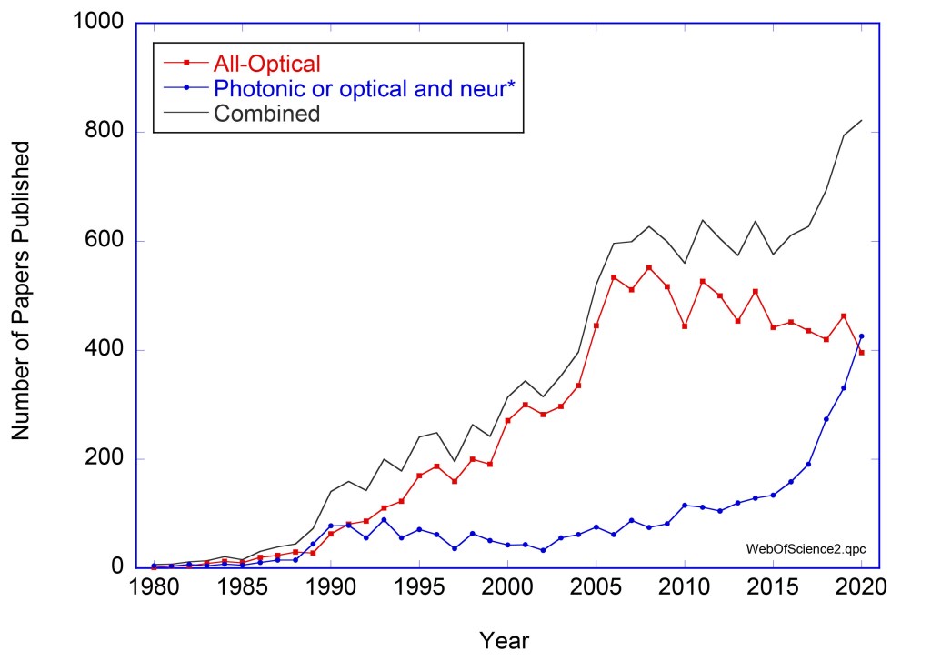
That said, it’s dangerous to ever say never, and research into all-optical computing and data processing is still going strong (See Fig. 1). It’s not the dream that was wrong, it was the time-scale that was wrong, just like fiber-to-the-home. Back in 2001, fiber-to-the-home was viewed as a pipe-dream by serious technology scouts. It took twenty years, but now that vision is coming true in urban settings. Back in 2001, all-optical computing seemed about 20 years away, but now it still looks 20 years out. Maybe this time the prediction is right. Recent advances in all-optical processing give some hope for it. Here are some of those advances.
Fig. 1 Number of papers published by year with the phrase in the title: “All-Optical” or “Photonic or Optical and Neur*” according to Web of Science search. The term “All-optical” saturated around 2005. Papers written around optical neural networks was low to 2015 but now is experiencing a strong surge. The sociology of title choices, and how favorite buzz words shift over time, can obscure underlying causes and trends, but overall there is current strong interest in all-optical systems.
The “What” and “Why” of All-Optical Processing
One of the great dreams of photonics is the use of light beams to perform optical logic in optical processors just as electronic currents perform electronic logic in transistors and integrated circuits.
Our information age, starting with the telegraph in the mid-1800’s, has been built upon electronics because the charge of the electron makes it a natural decision maker. Two charges attract or repel by Coulomb’s Law, exerting forces upon each other. Although we don’t think of currents acting in quite that way, the foundation of electronic logic remains electrical interactions.
But with these interactions also come constraints—constraining currents to be contained within wires, waiting for charging times that slow down decisions, managing electrical resistance and dissipation that generate heat (computer processing farms in some places today need to be cooled by glacier meltwater). Electronic computing is hardly a green technology.
Therefore, the advantages of optical logic are clear: broadcasting information without the need for expensive copper wires, little dissipation or heat, low latency (signals propagate at the speed of light). Furthermore, information on the internet is already in the optical domain, so why not keep it in the optical domain and have optical information packets making the decisions? All the routing and switching decisions about where optical information packets should go could be done by the optical packets themselves inside optical computers.
But there is a problem. Photons in free space don’t interact—they pass through each other unaffected. This is the opposite of what is needed for logic and decision making. The challenge of optical logic is then to find a way to get photons to interact.
Think of the scene in Star Wars: The New Hope when Obiwan Kenobi and Darth Vader battle to the death in a light saber duel—beams of light crashing against each other and repelling each other with equal and opposite forces. This is the photonic engineer’s dream! Light controlling light. But this cannot happen in free space. On the other hand, light beams can control other light beams inside nonlinear crystals where one light beam changes the optical properties of the crystal, hence changing how another light beam travels through it. These are nonlinear optical crystals.
Nonlinear Optics
Virtually all optical control designs, for any kind of optical logic or switch, require one light beam to affect the properties of another, and that requires an intervening medium that has nonlinear optical properties. The physics of nonlinear optics is actually simple: one light beam changes the electronic structure of a material which affects the propagation of another (or even the same) beam. The key parameter is the nonlinear coefficient that determines how intense the control beam needs to be to produce a significant modulation of the other beam. This is where the challenge is. Most materials have very small nonlinear coefficients, and the intensity of the control beam usually must be very high.
Fig. 2 Nonlinear optics: Light controlling light. Light does not interact in free space, but inside a nonlinear crystal, polarizability can create an effect interaction that can be surprisingly strong. Two-wave mixing (exchange of energy between laser beams) is shown in the upper pane. Optical associative holographic memory (four-wave mixing) is an example of light controlling light. The hologram is written when exposed by both “Light” and “Guang/Hikari”. When the recorded hologram is presented later only with “Guang/Hikari” it immediately translates it to “Light”, and vice versa.
Therefore, to create low-power all-optical logic gates and switches there are four main design principles: 1) increase the nonlinear susceptibility by engineering the material, 2) increase the interaction length between the two beams, 3) concentrate light into small volumes, and 4) introduce feedback to boost the internal light intensities. Let’s take these points one at a time.
Nonlinear susceptibility: The key to getting stronger interaction of light with light is in the ease with which a control beam of light can distort the crystal so that the optical conditions change for a signal beam. This is called the nonlinear susceptibility . When working with “conventional” crystals like semiconductors (e.g. CdZnSe) or rare-Earths (e.g. LiNbO3), there is only so much engineering that is possible to try to tweak the nonlinear susceptibilities. However, artificially engineered materials can offer significant increases in nonlinear susceptibilities, these include plasmonic materials, metamaterials, organic semiconductors, photonic crystals. An increasingly important class of nonlinear optical devices are semiconductor optical amplifiers (SOA).
Interaction length: The interaction strength between two light waves is a product of the nonlinear polarization and the length over which the waves interact. Interaction lengths can be made relatively long in waveguides but can be made orders of magnitude longer in fibers. Therefore, nonlinear effects in fiber optics are a promising avenue for achieving optical logic.
Intensity Concentration: Nonlinear polarization is the product of the nonlinear susceptibility with the field amplitude of the waves. Therefore, focusing light down to small cross sections produces high power, as in the core of a fiber optic, again showing advantages of fibers for optical logic implementations.
Feedback: Feedback, as in a standing-wave cavity, increases the intensity as well as the effective interaction length by folding the light wave continually back on itself. Both of these effects boost the nonlinear interaction, but then there is an additional benefit: interferometry. Cavities, like a Fabry-Perot, are interferometers in which a slight change in the round-trip phase can produce large changes in output light intensity. This is an optical analog to a transistor in which a small control current acts as a gate for an exponential signal current. The feedback in the cavity of a semiconductor optical amplifier (SOA), with high internal intensities and long effective interaction lengths and an active medium with strong nonlinearity make these elements attractive for optical logic gates. Similarly, integrated ring resonators have the advantage of interferometric control for light switching. Many current optical switches and logic gates are based on SOAs and integrated ring resonators.
All-Optical Regeneration
The vision of the all-optical internet, where the logic operations that direct information to different locations is all performed by optical logic without ever converting into the electrical domain, is facing a barrier that is as challenging to overcome today as it was back in 2001: all-optical regeneration. All-optical regeneration has been and remains the Achilles Heal of the all-optical internet.
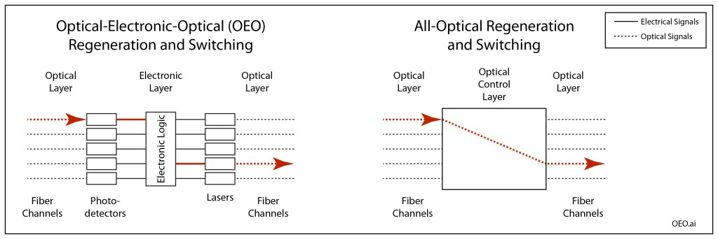
Signal regeneration is currently performed through OEO conversion: Optical-to-Electronic-to-Optical. In OEO conversion, a distorted signal (distortion is caused by attenuation and dispersion and noise as signals travel down fiber optics) is received by a photodetector, is interpreted as ones and zeros that drive laser light sources that launch the optical pulses down the next stretch of fiber. The new pulses are virtually perfect, but they again degrade as they travel, until they are regenerated, and so on. The added advantage of the electrical layer is that the electronic signals can be used to drive conventional electronic logic for switching.
In all-optical regeneration, on the other hand, the optical pulses need to be reamplified, reshaped and retimed––known as 3R regeneration––all by sending the signal pulses through nonlinear amplifiers and mixers, which may include short stretches of highly nonlinear fiber (HNLF) or semiconductor optical amplifiers (SOA). There have been demonstrations of 2R all-optical regeneration (reamplifying and reshaping but not retiming) at lower data rates, but getting all 3Rs at the high data rates (40 Gb/s) in the next generation telecom systems remains elusive.
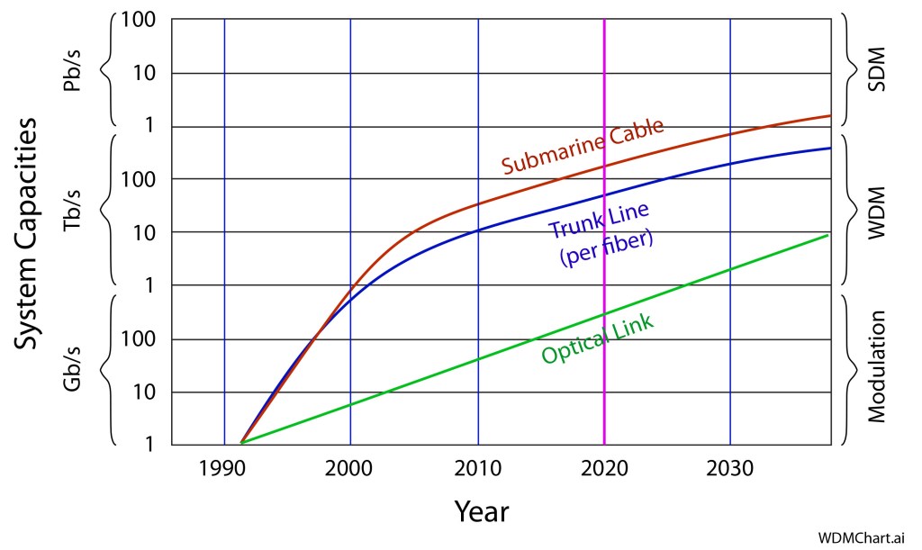
Nonetheless, there is an active academic literature that is pushing the envelope on optical logical devices and regenerators [1]. Many of the systems focus on SOA’s, HNLF’s and Interferometers. Numerical modeling of these kinds of devices is currently ahead of bench-top demonstrations, primarily because of the difficulty of fabrication and device lifetime. But the numerical models point to performance that would be competitive with OEO. If this OOO conversion (Optical-to-Optical-to-Optical) is scalable (can handle increasing bit rates and increasing numbers of channels), then the current data crunch that is facing the telecom trunk lines (see my previous Blog) may be a strong driver to implement such all-optical solutions.
It is important to keep in mind that legacy technology is not static but also continues to improve. As all-optical logic and switching and regeneration make progress, OEO conversion gets incrementally faster, creating a moving target. Therefore, we will need to wait another 20 years to see whether OEO is overtaken and replaced by all-optical.
Fig. 3 Optical-Electronic-Optical regeneration and switching compared to all-optical control. The optical control is performed using SOA’s, interferometers and nonlinear fibers.
Photonic Neural Networks
The most exciting area of optical logic today is in analog optical computing––specifically optical neural networks and photonic neuromorphic computing [2, 3]. A neural network is a highly-connected network of nodes and links in which information is distributed across the network in much the same way that information is distributed and processed in the brain. Neural networks can take several forms––from digital neural networks that are implemented with software on conventional digital computers, to analog neural networks implemented in specialized hardware, sometimes also called neuromorphic computing systems.
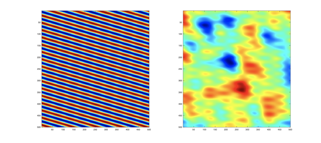
Optics and photonics are well suited to the analog form of neural network because of the superior ability of light to form free-space interconnects (links) among a high number of optical modes (nodes). This essential advantage of light for photonic neural networks was first demonstrated in the mid-1980’s using recurrent neural network architectures implemented in photorefractive (nonlinear optical) crystals (see Fig. 1 for a publication timeline). But this initial period of proof-of-principle was followed by a lag of about 2 decades due to a mismatch between driver applications (like high-speed logic on an all-optical internet) and the ability to configure the highly complex interconnects needed to perform the complex computations.
Fig. 4 Optical vector-matrix multiplication. An LED array is the input vector, focused by a lens onto the spatial light modulator that is the 2D matrix. The transmitted light is refocussed by the lens onto a photodiode array with is the output vector. Free-space propagation and multiplication is a key advantage to optical implementation of computing.
The rapid rise of deep machine learning over the past 5 years has removed this bottleneck, and there has subsequently been a major increase in optical implementations of neural networks. In particular, it is now possible to use conventional deep machine learning to design the interconnects of analog optical neural networks for fixed tasks such as image recognition [4]. At first look, this seems like a non-starter, because one might ask why not use the conventional trained deep network to do the recognition itself rather than using it to create a special-purpose optical recognition system. The answer lies primarily in the metrics of latency (speed) and energy cost.
In neural computing, approximately 90% of the time and energy go into matrix multiplication operations. Deep learning algorithms driving conventional digital computers need to do the multiplications at the sequential clock rate of the computer using nested loops. Optics, on the other had, is ideally suited to perform matrix multiplications in a fully parallel manner (see Fig. 4). In addition, a hardware implementation using optics operates literally at the speed of light. The latency is limited only by the time of flight through the optical system. If the optical train is 1 meter, then the time for the complete computation is only a few nanoseconds at almost no energy dissipation. Combining the natural parallelism of light with the speed has led to unprecedented computational rates. For instance, recent implementations of photonic neural networks have demonstrated over 10 Trillion operations per second (TOPS) [5].
It is important to keep in mind that although many of these photonic neural networks are characterized as all-optical, they are generally not reconfigurable, meaning that they are not adaptive to changing or evolving training sets or changing input information. Most adaptive systems use OEO conversion with electronically-addressed spatial light modulators (SLM) that are driven by digital logic. Another technology gaining recent traction is neuromorphic photonics in which neural processing is implemented on photonic integrated circuits (PICS) with OEO conversion. The integration of large numbers of light emitting sources on PICs is now routine, relieving the OEO bottleneck as electronics and photonics merge in silicon photonics.
Farther afield are all-optical systems that are adaptive through the use of optically-addressed spatial light modulators or nonlinear materials. In fact, these types of adaptive all-optical neural networks were among the first demonstrated in the late 1980’s. More recently, advanced adaptive optical materials, as well as fiber delay lines for a type of recurrent neural network known as reservoir computing, have been used to implement faster and more efficient optical nonlinearities needed for adaptive updates of neural weights. But there are still years to go before light is adaptively controlling light entirely in the optical domain at the speeds and with the flexibility needed for real-world applications like photonic packet switching in telecom fiber-optic routers.
In stark contrast to the status of classical all-optical computing, photonic quantum computing is on the cusp of revolutionizing the field of quantum information science. The recent demonstration from the Canadian company Xanadu of a programmable photonic quantum computer that operates at room temperature may be the harbinger of what is to come in the third generation Machines of Light: Quantum Optical Computers, which is the topic of my next blog.
By David D. Nolte, Nov. 28, 2021
Further Reading
[1] V. Sasikala and K. Chitra, “All optical switching and associated technologies: a review,” Journal of Optics-India, vol. 47, no. 3, pp. 307-317, Sep (2018)
[2] C. Huang et a., “Prospects and applications of photonic neural networks,” Advances in Physics-X, vol. 7, no. 1, Jan (2022), Art no. 1981155
[5] X. Y. Xu, M. X. Tan, B. Corcoran, J. Y. Wu, A. Boes, T. G. Nguyen, S. T. Chu, B. E. Little, D. G. Hicks, R. Morandotti, A. Mitchell, and D. J. Moss, “11 TOPS photonic convolutional accelerator for optical neural networks,” Nature, vol. 589, no. 7840, pp. 44-+, Jan (2021)
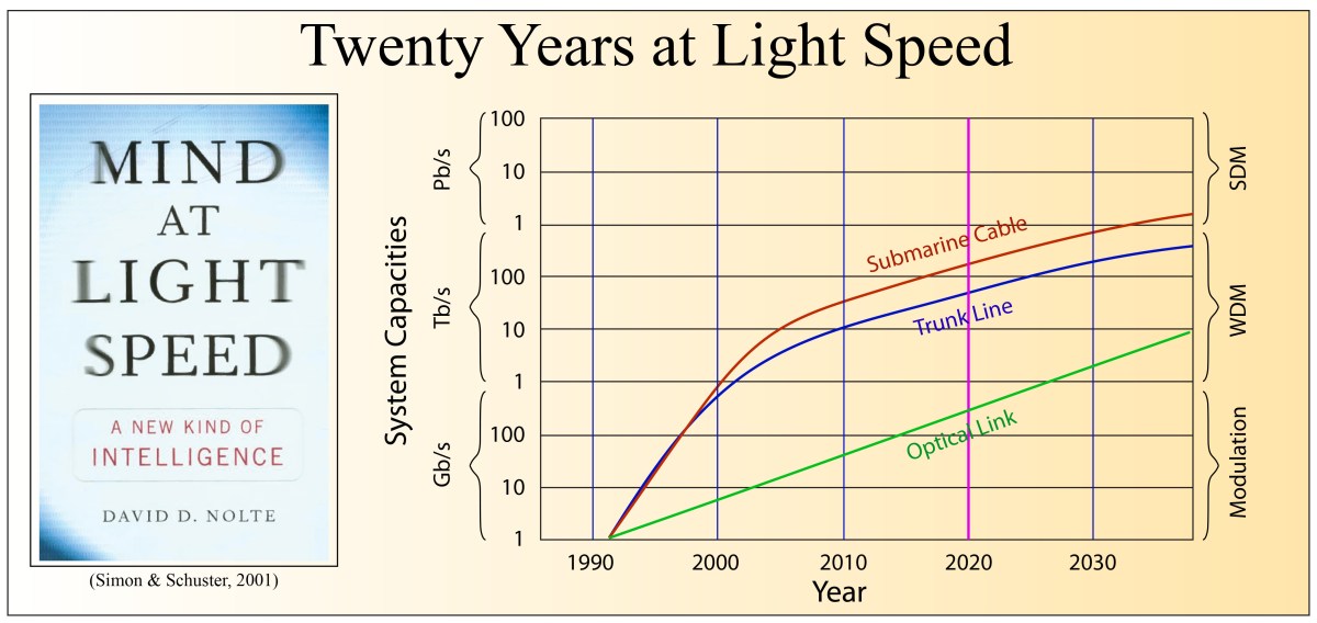
Twenty years ago this November, my book Mind at Light Speed: A New Kind of Intelligence was published by The Free Press (Simon & Schuster, 2001). The book described the state of optical science at the turn of the Millennium through three generations of Machines of Light: The Optoelectronic Generation of electronic control meshed with photonic communication; The All-Optical Generation of optical logic; and The Quantum Optical Generation of quantum communication and computing.
To mark the occasion of the publication, this Blog Post begins a three-part series that updates the state-of-the-art of optical technology, looking at the advances in optical science and technology over the past 20 years since the publication of Mind at Light Speed. This first blog reviews fiber optics and the photonic internet. The second blog reviews all-optical communication and computing. The third and final blog reviews the current state of photonic quantum communication and computing.
The Wabash Yacht Club
During late 1999 and early 2000, while I was writing Mind at Light Speed, my wife Laura and I would often have lunch at the ironically-named Wabash Yacht Club. Not only was it not a Yacht Club, but it was a dark and dingy college-town bar located in a drab 70-‘s era plaza in West Lafayette, Indiana, far from any navigable body of water. But it had a great garlic burger and we loved the atmosphere.
One of the TV monitors in the bar was always tuned to a station that covered stock news, and almost every day we would watch the NASDAQ rise 100 points just over lunch. This was the time of the great dot-com stock-market bubble—one of the greatest speculative bubbles in the history of world economics. In the second quarter of 2000, total US venture capital investments exceeded $30B as everyone chased the revolution in consumer market economics.
Fiber optics will remain the core technology of the internet for the foreseeable future.
Part of that dot-com bubble was a massive bubble in optical technology companies, because everyone knew that the dot-com era would ride on the back of fiber optics telecommunications. Fiber optics at that time had already revolutionized transatlantic telecommunications, and there seemed to be no obstacle for it to do the same land-side with fiber optics to every home bringing every dot-com product to every house and every movie ever made. What would make this possible was the tremendous information bandwidth that can be crammed into tiny glass fibers in the form of photon packets traveling at the speed of light.
Doing optics research at that time was a heady experience. My research on real-time optical holography was only on the fringe of optical communications, but at the CLEO conference on lasers and electro-optics, I was invited by tiny optics companies to giant parties, like a fully-catered sunset cruise on a schooner sailing Baltimore’s inner harbor. Venture capital scouts took me to dinner in San Francisco with an eye to scoop up whatever patents I could dream of. And this was just the side show. At the flagship fiber-optics conference, the Optical Fiber Conference (OFC) of the OSA, things were even crazier. One tiny company that made a simple optical switch went almost overnight from a company worth a couple of million to being bought out by Nortel (the giant Canadian telecommunications conglomerate of the day) for over 4 billion dollars.
The Telecom Bubble and Bust
On the other side from the small mom-and-pop optics companies were the giants like Corning (who made the glass for the glass fiber optics) and Nortel. At the height of the telecom bubble in September 2000, Nortel had a capitalization of almost $400B Canadian dollars due to massive speculation about the markets around fiber-optic networks.
One of the central questions of the optics bubble of Y2K was what the new internet market would look like. Back then, fiber was only beginning to connect to distribution nodes that were connected off the main cross-country trunk lines. Cable TV dominated the market with fixed programming where you had to watch whatever they transmitted whenever they transmitted it. Google was only 2 years old, and Youtube didn’t even exist then—it was founded in 2005. Everyone still shopped at malls, while Amazon had only gone public three years before.
There were fortune tellers who predicted that fiber-to-the-home would tap a vast market of online commerce where you could buy anything you wanted and have it delivered to your door. They foretold of movies-on-demand, where anyone could stream any movie they wanted at any time. They also foretold of phone calls and video chats that never went over the phone lines ruled by the telephone monopolies. The bandwidth, the data rates, that these markets would drive were astronomical. The only technology at that time that could support such high data rates was fiber optics.
At first, these fortune tellers drove an irrational exuberance. But as the stocks inflated, there were doomsayers who pointed out that the costs at that time of bringing fiber into homes was prohibitive. And the idea that people would be willing to pay for movies-on-demand was laughable. The cost of the equipment and the installation just didn’t match what then seemed to be a sparse market demand. Furthermore, the fiber technology in the year 2000 couldn’t even get to the kind of data rates that could support these dreams.
In March of 2000 the NASDAQ hit a high of 5000, and then the bottom fell out.
By November 2001 the NASDAQ had fallen to 1500. One of the worst cases of the telecom bust was Nortel whose capitalization plummeted from $400B at its high to $5B Canadian by August 2002. Other optics companies fared little better.
The main questions, as we stand now looking back from 20 years in the future, are: What in real life motivated the optics bubble of 2000? And how far has optical technology come since then? The surprising answer is that the promise of optics in 2000 was not wrong—the time scale was just off.
Fiber to the Home
Today, fixed last-mile broadband service is an assumed part of life in metro areas in the US. This broadband takes on three forms: legacy coaxial cable, 4G wireless soon to be upgraded to 5G, and fiber optics. There are arguments pro and con for each of these technologies, especially moving forward 10 or 20 years or more, and a lot is at stake. The global market revenue was $108 Billion in 2020 and is expected to reach $200 Billion in 2027, growing at over 9% from 2021 to 2027.
(ShutterStock_75369058.jpg)
To sort through the pros and cons to pick the wining technology, several key performance parameters must be understood for each technology. The two most important performance measures are bandwidth and latency. Bandwidth is the data rate—how many bits per second can you get to the home. Latency is a little more subtle. It is the time it takes to complete a transmission. This time includes the actual time for information to travel from a transmitter to a receiver, but that is rarely the major contributor. Currently, almost all of the latency is caused by the logical operations needed to move the information onto and off of the home data links.
Coax (short for coaxial cable) is attractive because so much of the last-mile legacy hardware is based on the old cable services. But coax cable has very limited bandwidth and high latency. As a broadband technology, it is slowly disappearing.
Wireless is attractive because the information is transmitted in the open air without any need for physical wires or fibers. But high data rates require high frequency. For instance, 4G wireless operates at frequencies between 700 MHz to 2.6 GHz. Current WiFi is 2.4 GHz or 5 GHz, and next-generation 5G will have 26 GHz using millimeter wave technology, and WiGig is even more extreme at 60 GHz. While WiGig will deliver up to 10 Gbits per second, as everyone with wireless routers in their homes knows, the higher the frequency, the more it is blocked by walls or other obstacles. Even 5 GHz is mostly attenuated by walls, and the attenuation gets worse as the frequency gets higher. Testing of 5G networks has shown that cell towers need to be closely spaced to allow seamless coverage. And the crazy high frequency of WiGig all but guarantees that it will only be usable for line-of-sight communication within a home or in an enterprise setting.
Fiber for the last mile, on the other hand, has multiple advantages. Chief among these is that fiber is passive. It is a light pipe that has ten thousand times more usable bandwidth than a coaxial cable. For instance, lab tests have pushed up to 100 Tbit/sec over kilometers of fiber. To access that bandwidth, the input and output hardware can be continually upgraded, while the installed fiber is there to handle pretty much any amount of increasing data rates for the next 10 or 20 years. Fiber installed today is supporting 1 Gbit/sec data rates, and the existing protocol will work up to 10 Gbit/sec—data rates that can only be hoped for with WiFi. Furthermore, optical communications on fiber have latencies of around 1.5 msec over 20 kilometers compared with 4G LTE that has a latency of 8 msec over 1 mile. The much lower latency is key to support activities that cannot stand much delay, such as voice over IP, video chat, remote controlled robots, and virtual reality (i.e., gaming). On top of all of that, the internet technology up to the last mile is already almost all optical. So fiber just extends the current architecture across the last mile.
Therefore, fixed fiber last-mile broadband service is a technology winner. Though the costs can be higher than for WiFi or coax in the short run for installation, the long-run costs are lower when amortized over the lifetime of the installed fiber which can exceed 25 years.
It is becoming routine to have fiber-to-the-curb (FTTC) where a connection box converts photons in fibers into electrons on copper to take the information into the home. But a market also exists in urban settings for fiber-to-the-home (FTTH) where the fiber goes directly into the house to a receiver and only then would the information be converted from photons to electrons and electronics.
Shortly after Mind at Light Speed was published in 2001, I was called up by a reporter for the Seattle Times who wanted to know my thoughts about FTTH. When I extolled its virtue, he nearly hung up on me. He was in the middle of debunking the telecom bubble and his premise was that FTTH was a fraud. In 2001 he might have been right. But in 2021, FTTH is here, it is expanding, and it will continue to do so for at least another quarter century. Fiber to the home will become the legacy that some future disruptive technology will need to displace.
Fig. 1 Optical data rates on optical links, trunk lines and submarine cables over the past 30 years and projecting into the future. Redrawn from Refs. [1, 2]
Trunk-Line Fiber Optics
Despite the rosy picture for Fiber to the Home, a storm is brewing for the optical trunk lines. The total traffic on the internet topped a billion Terrabytes in 2019 and is growing fast, doubling about every 2 years on an exponential growth curve. In 20 years, that becomes another factor of a thousand more traffic in 2040 than today. Therefore, the technology companies that manage and supply the internet worry about a capacity crunch that is fast approaching when there will be more demand than the internet can supply.
Over the past 20 years, the data rates on the fiber trunk lines—the major communication links that span the United States—matched demand by packing more bits in more ways into the fibers. Up to 2009, increased data rates were achieved using dispersion-managed wavelength-division multiplexing (WDM) which means that they kept adding more lasers of slightly different colors to send the optical bits down the fiber. For instance, in 2009 the commercial standard was 80 colors each running at 40 Gbit/sec for a total of 3.2 Tbit/sec down a single fiber.
Since 2009, increased bandwidth has been achieved through coherent WDM, where not only the amplitude of light but also the phase of the light is used to encode bits of information using interferometry. We are still in the coherent WDM era as improved signal processing is helping to fill the potential coherent bandwidth of a fiber. Commercial protocols using phase-shift keying, quadrature phase-shift keying, and 16-quadrature amplitude modulation currently support 50 Gbit/sec, 100 Gbit/sec and 200 Gbit/sec, respectively. But the capacity remaining is shrinking, and several years from now, a new era will need to begin in order to keep up with demand. But if fibers are already using time, color, polarization and phase to carry information, what is left?
The answer is space!
Coming soon will be commercial fiber trunk lines that use space-division multiplexing (SDM). The simplest form is already happening now as fiber bundles are replacing single-mode fibers. If you double the number of fibers in a cable, then you double the data rate of the cable. But the problem with this simple approach is the scaling. If you double just 10 times, then you need 1024 fibers in a single cable—each fiber needing its own hardware to launch the data and retrieve it at the other end. This is linear scaling, which is bad scaling for commercial endeavors.
Fig. 2 Fiber structures for space-division multiplexing (SDM). Fiber bundles are cables of individual single-mode fibers. Multi-element fibers (MEF) are single-mode fibers formed together inside the coating. Multi-core fibers (MCF) have multiple cores within the cladding. Few-mode fibers (FMF) are multi-mode fibers with small mode numbers. Coupled core (CC) fibers are multi-core fibers in which the cores are close enough that the light waves are coupled into coupled spatial modes. Redrawn from Ref. [3]
Therefore, alternatives for tapping into SDM are being explored in lab demonstrations now that have sublinear scaling (costs don’t rise as fast as improved capacity). These include multi-element fibers where multiple fiber optical elements are manufactured as a group rather than individually and then combined into a cable. There are also multi-core fibers, where multiple fibers share the same cladding. These approaches provide multiple fibers for multiple channels without a proportional rise in cost.
More exciting are approaches that use few-mode-fibers (FMF) to support multiple spatial modes traveling simultaneously down the same fiber. In the same vein are coupled-core fibers which is a middle ground between multi-core fibers and few-mode fibers in that individual cores can interact within the cladding to support coupled spatial modes that can encode separate spatial channels. Finally, combinations of approaches can use multiple formats. For instance, a recent experiment combined FMF and MCF that used 19 cores each supporting 6 spatial modes for a total of 114 spatial channels.
However, space-division multiplexing has been under development for several years now, yet it has not fully moved into commercial systems. This may be a sign that the doubling rate of bandwidth may be starting to slow down, just as Moore’s Law slowed down for electronic chips. But there were doomsayers foretelling the end of Moore’s Law for decades before it actually slowed down, because new ideas cannot be predicted. But even if the full capacity of fiber is being approached, there is certainly nothing that will replace fiber with any better bandwidth. So fiber optics will remain the core technology of the internet for the foreseeable future.
But what of the other generations of Machines of Light: the all-optical and the quantum-optical generations? How have optics and photonics fared in those fields? Stay tuned for my next blogs to find out.
By David D. Nolte, Nov. 8, 2021
Bibliography
[1] P. J. Winzer, D. T. Neilson, and A. R. Chraplyvy, “Fiber-optic transmission and networking: the previous 20 and the next 20 years,” Optics Express, vol. 26, no. 18, pp. 24190-24239, Sep (2018) [Link]
[2] W. Shi, Y. Tian, and A. Gervais, “Scaling capacity of fiber-optic transmission systems via silicon photonics,” Nanophotonics, vol. 9, no. 16, pp. 4629-4663, Nov (2020)
[3] E. Agrell, M. Karlsson, A. R. Chraplyvy, D. J. Richardson, P. M. Krummrich, P. Winzer, K. Roberts, J. K. Fischer, S. J. Savory, B. J. Eggleton, M. Secondini, F. R. Kschischang, A. Lord, J. Prat, I. Tomkos, J. E. Bowers, S. Srinivasan, M. Brandt-Pearce, and N. Gisin, “Roadmap of optical communications,” Journal of Optics, vol. 18, no. 6, p. 063002, 2016/05/04 (2016) [Link]
If you have ever seen euphemistically-named “snow”—the black and white dancing pixels on television screens in the old days of cathode-ray tubes—you may think it is nothing but noise. But the surprising thing about noise is that it is a good place to hide information.
Shine a laser pointer on any rough surface and look at the scattered light on a distant wall, then you will see the same patterns of light and dark known as laser speckle. If you move your head or move the pointer, then the speckle shimmers—just like the snow on the old TVs. This laser speckle—this snow—is providing fundamental new ways to extract information hidden inside three-dimensional translucent objects—objects like biological tissue or priceless paintings or silicon chips.
Snow Crash
The science fiction novel Snow Crash, published in 1992 by Neal Stephenson, is famous for popularizing virtual reality and the role of avatars. The central mystery of the novel is the mind-destroying mental crash that is induced by Snow—white noise in the metaverse. The protagonist hero of the story—a hacker with an avatar improbably named Hiro Protagonist—must find the source of snow and thwart the nefarious plot behind it.
Fig. 1 Book cover of Snow Crash
If Hiro’s snow in his VR headset is caused by laser speckle, then the seemingly random pattern is composed of amplitudes and phases that vary spatially and temporally. There are many ways to make computer-generated versions of speckle. One of the simplest is to just add together a lot of sinusoidal functions with varying orientations and periodicities. This is a “Fourier” approach to speckle which views it as a random superposition of two-dimensional spatial frequencies. An example is shown in Fig. 2 for one sinusoid which has been added to 20 others to generate the speckle pattern on the right. There is still residual periodicity in the speckle for N = 20, but as N increases, the speckle pattern becomes strictly random, like noise.
But if the sinusoids that are being added together link the periodicity with their amplitude through some functional relationship, then the final speckle can be analyze using a 2D Fourier transform to find its spatial frequency spectrum. The functional form of this spectrum can tell a lot about the underlying processes of the speckle formation. This is part of the information hidden inside snow.
Fig. 2 Sinusoidal addition to generate random speckle. a) One example of a spatial periodicity. b) The superposition of 20 random sinusoids.
An alternative viewpoint to generating a laser speckle pattern thinks in terms of spatially-localized patches that add randomly together with random amplitudes and phases. This is a space-domain view of speckle formation in contrast to the Fourier-space view of the previous construction. Sinusoids are “global” extending spatially without bound. The underlying spatially localized functions can be almost any local function. Gaussians spring to mind, but so do Airy functions, because they are common point-spread functions that participate in the formation of images through lenses. The example in Fig 3a shows one such Airy function, and in 3b for speckle generated from N = 20 Airy functions of varying amplitudes and phases and locations.
Fig. 3 Generating speckle by random superposition of point spread functions (spatially-localized functions) of varying amplitude, phase, position and bandwidth.
These two examples are complementary ways of generating speckle, where the 2D Fourier-domain approach is conjugate to the 2D space-domain approach.
However, laser speckle is actually a 3D phenomenon, and the two-dimensional speckle patterns are just 2D cross sections intersecting a complex 3D pattern of light filaments. To get a sense of how laser speckle is formed in a physical system, one can solve the propagation of a laser beam through a random optical medium. In this way you can visualize the physical formation of the regions of brightness and darkness when the fragmented laser beam exits the random material.
Fig. 4 Propagation of a coherent beam into a random optical medium. Speckle is intrinsically three dimensional while 2D speckle is the cross section of the light filaments.
Coherent Patch
For a quantitative understanding of laser speckle, when 2D laser speckle is formed by an optical system, the central question is how big are the regions of brightness and darkness? This is a question of spatial coherence, and one way to define spatial coherence is through the coherence area at the observation plane
where A is the source emitting area, z is the distance to the observation plane, and Ωs is the solid angle subtended by the source emitting area as seen from the observation point. This expression assumes that the angular spread of the light scattered from the illumination area is very broad. Larger distances and smaller emitting areas (pinholes in an optical diffuser or focused laser spots on a rough surface) produce larger coherence areas in the speckle pattern. For a Gaussian intensity distribution at the emission plane, the coherence area is
for beam waist w0 at the emission plane. To put some numbers to these parameters to give an intuitive sense of the size of speckle spots, assume a wavelength of 1 micron, a focused beam waist of 0.1 mm and a viewing distance of 1 meter. This gives patches with a radius of about 2 millimeters. Examples of laser speckle are shown in Fig. 5 for a variety of beam waist values w0.
Fig. 5 Speckle intensities for Gaussian illumination of a random phase screen for changing illumination radius w0 = 64, 32, 16 and 8 microns for f = 1 cm and W = 500 nm with a field-of-view of 5 mm. (Reproduced from Ref.[1])
Speckle Holograms
Associated with any intensity modulation must be a phase modulation through the Kramers-Kronig relations [2]. Phase cannot be detected directly in the speckle intensity pattern, but it can be measured by using interferometry. One of the easiest interferometric techniques is holography in which a coherent plane wave is caused to intersect, at a small angle, a speckle pattern generated from the same laser source. An example of a speckle hologram and its associated phase is shown in Fig. 6. The fringes of the hologram are formed when a plane reference wave interferes with the speckle field. The fringes are not parallel because of the varying phase of the speckle field, but the average spatial frequency is still recognizable in Fig. 5a. The associated phase map is shown in Fig. 5b.
Fig. 6 Speckle hologram and speckle phase. a) A coherent plane-wave reference added to fully-developed speckle (unity contrast) produces a speckle hologram. b) The phase of the speckle varies through 2π.
Optical Vortex Physics
In the speckle intensity field, there are locations where the intensity vanishes, and the phase becomes undefined. In the neighborhood of a singular point the phase wraps around it with a 2pi phase range. Because of the wrapping phase such a singular point is called and optical vortex [3]. Vortices always come in pairs with opposite helicity (defined by the direction of the wrapping phase) with a line of neutral phase between them as shown in Fig. 7. The helicity defines the topological charge of the vortex, and they can have topological charges larger than ±1 if the phase wraps multiple times. In dynamic speckle these vortices are also dynamic and move with speeds related to the underlying dynamics of the scattering medium [4]. Vortices can annihilate if they have opposite helicity, and they can be created in pairs. Studies of singular optics have merged with structured illumination [5] to create an active field of topological optics with applications in biological microscopy as well as material science.
iFig. 7 Optical vortex patterns. a) Log intensity showing zeros in the intensity field. The circles identify the intensity nulls which are the optical vortices b) Associated phase with a 2pi phase wrapping around each singularity. c) Associated hologram showing dislocations in the fringes that occur at the vortices.
References
[1] D. D. Nolte, Optical Interferometry for Biology and Medicine. (Springer, 2012)
[2] A. Mecozzi, C. Antonelli, and M. Shtaif, “Kramers-Kronig coherent receiver,” Optica, vol. 3, no. 11, pp. 1220-1227, Nov (2016)
[3] M. R. Dennis, R. P. King, B. Jack, K. O’Holleran, and M. J. Padgett, “Isolated optical vortex knots,” Nature Physics, vol. 6, no. 2, pp. 118-121, Feb (2010)
[4] S. J. Kirkpatrick, K. Khaksari, D. Thomas, and D. D. Duncan, “Optical vortex behavior in dynamic speckle fields,” Journal of Biomedical Optics, vol. 17, no. 5, May (2012), Art no. 050504
[5] H. Rubinsztein-Dunlop, A. Forbes, M. V. Berry, M. R. Dennis, D. L. Andrews, M. Mansuripur, C. Denz, C. Alpmann, P. Banzer, T. Bauer, E. Karimi, L. Marrucci, M. Padgett, M. Ritsch-Marte, N. M. Litchinitser, N. P. Bigelow, C. Rosales-Guzman, A. Belmonte, J. P. Torres, T. W. Neely, M. Baker, R. Gordon, A. B. Stilgoe, J. Romero, A. G. White, R. Fickler, A. E. Willner, G. D. Xie, B. McMorran, and A. M. Weiner, “Roadmap on structured light,” Journal of Optics, vol. 19, no. 1, Jan (2017), Art no. 013001
One of the hardest aspects to grasp about relativity theory is the question of whether an event “looks as if” it is doing something, or whether it “actually is” doing something.
Take, for instance, the classic twin paradox of relativity theory in which there are twins who wear identical high-precision wrist watches. One of them rockets off to Alpha Centauri at relativistic speeds and returns while the other twin stays on Earth. Each twin sees the other twin’s clock running slowly because of relativistic time dilation. Yet when they get back together and, standing side-by-side, they compare their watches—the twin who went to Alpha Centauri is actually younger than the other, despite the paradox. The relativistic effect of time dilation is “real”, not just apparent, regardless of whether they come back together to do the comparison.
Yet this understanding of relativistic effects took many years, even decades, to gain acceptance after Einstein proposed them. He was aware himself that key experiments were required to prove that relativistic effects are real and not just apparent.
Einstein and the Transverse Doppler Effect
In 1905 Einstein used his new theory of special relativity to predict observable consequences that included relativistic velocity addition and a general treatment of the relativistic Doppler effect [1]. This included the effects of time dilation in addition to the longitudinal effect of the source chasing the wave. Time dilation produced a correction to Doppler’s original expression for the longitudinal effect that became significant at speeds approaching the speed of light. More significantly, it predicted a transverse Doppler effect for a source moving along a line perpendicular to the line of sight to an observer. This effect had not been predicted either by Christian Doppler (1803 – 1853) or by Woldemar Voigt (1850 – 1919).
Despite the generally positive reception of Einstein’s theory of special relativity, some of its consequences were anathema to many physicists at the time. A key stumbling block was the question whether relativistic effects, like moving clocks running slowly, were only apparent, or were actually real, and Einstein had to fight to convince others of its reality. When Johannes Stark (1874 – 1957) observed Doppler line shifts in ion beams called “canal rays” in 1906 (Stark received the 1919 Nobel prize in part for this discovery) [3], Einstein promptly published a paper suggesting how the canal rays could be used in a transverse geometry to directly detect time dilation through the transverse Doppler effect [4]. Thirty years passed before the experiment was performed with sufficient accuracy by Herbert Ives and G. R. Stilwell in 1938 to measure the transverse Doppler effect [5]. Ironically, even at this late date, Ives and Stilwell were convinced that their experiment had disproved Einstein’s time dilation by supporting Lorentz’ contraction theory of the electron. The Ives-Stilwell experiment was the first direct test of time dilation, followed in 1940 by muon lifetime measurements [6].
A) Transverse Doppler Shift Relative to EmissionAngle
The Doppler effect varies between blue shifts in the forward direction to red shifts in the backward direction, with a smooth variation in Doppler shift as a function of the emission angle. Consider the configuration shown in Fig. 1 for light emitted from a source moving at speed v and emitting at an angle θ0 in the receiver frame. The source moves a distance vT in the time of a single emission cycle (assume a harmonic wave). In that time T (which is the period of oscillation of the light source — or the period of a clock if we think of it putting out light pulses) the light travels a distance cT before another cycle begins (or another pulse is emitted).
Fig. 1 Configuration for detection of Doppler shifts for emission angle θ0. The light source travels a distance vT during the time of a single cycle, while the wavefront travels a distance cT towards the detector.
The observed wavelength in the receiver frame is thus given by
where T is the emission period of the moving source. Importantly, the emission period is time dilated relative to the proper emission time of the source
Therefore,
This expression can be evaluated for several special cases:
a) θ0 = 0 for forward emission
which is the relativistic blue shift for longitudinal motion in the direction of the receiver.
b) θ0 = π for backward emission
which is the relativistic red shift for longitudinal motion away from the receiver
c) θ0 = π/2 for transverse emission
This transverse Doppler effect for emission at right angles is a red shift, caused only by the time dilation of the moving light source. This is the effect proposed by Einstein and observed by Stark that proved moving clocks tick slowly. But it is not the only way to view the transverse Doppler effect.
B) Transverse Doppler Shift Relative to Angle at Reception
A different option for viewing the transverse Doppler effect is the angle to the moving source at the moment that the light is detected. The geometry of this configuration relative to the previous is illustrated in Fig. 2.
Fig. 2 The detection point is drawn at a finite distance. However, the relationship between θ0 and θ1 is independent of the distance to the detector
The transverse distance to the detection point is
The length of the line connecting the detection point P with the location of the light source at the moment of detection is (using the law of cosines)
Combining with the first equation gives
An equivalent expression is obtained as
Note that this result, relating θ1 to θ0, is independent of the distance to the observation point.
When θ1 = π/2, then
yielding
for which the Doppler effect is
which is a blue shift. This creates the unexpected result that sin θ0 = π/2 produces a red shift, while sin θ1 = π/2 produces a blue shift. The question could be asked: which one represents time dilation? In fact, it is sin θ0 = π/2 that produces time dilation exclusively, because in that configuration there is no foreshortening effect on the wavelength–only the emission time.
C) Compromise: The Null Transverse Doppler Shift
The previous two configurations each could be used as a definition for the transverse Doppler effect. But one gives a red shift and one gives a blue shift, which seems contradictory. Therefore, one might try to strike a compromise between these two cases so that sin θ1 = sin θ0, and the configuration is shown in Fig. 3.
This is the case when θ1 + θ2 = π. The sines of the two angles are equal, yielding
and
which is solved for
Inserting this into the Doppler equation gives
where the Taylor’s expansion of the denominator (at low speed) cancels the numerator to give zero net Doppler shift. This compromise configuration represents the condition of null Doppler frequency shift. However, for speeds approaching the speed of light, the net effect is a lengthening of the wavelength, dominated by time dilation, causing a red shift.
D) Source in Circular Motion Around Receiver
An interesting twist can be added to the problem of the transverse Doppler effect: put the source or receiver into circular motion, one about the other. In the case of a source in circular motion around the receiver, it is easy to see that this looks just like case A) above for θ0 = π/2, which is the red shift caused by the time dilation of the moving source
However, there is the possible complication that the source is no longer in an inertial frame (it experiences angular acceleration) and therefore it is in the realm of general relativity instead of special relativity. In fact, it was Einstein’s solution to this problem that led him to propose the Equivalence Principle and make his first calculations on the deflection of light by gravity. His solution was to think of an infinite number of inertial frames, each of which was instantaneously co-moving with the same linear velocity as the source. These co-moving frames are inertial and can be analyzed using the principles of special relativity. The general relativistic effects come from slipping from one inertial co-moving frame to the next. But in the case of the circular transverse Doppler effect, each instantaneously co-moving frame has the exact configuration as case A) above, and so the wavelength is red shifted exactly by the time dilation.
Fig. Left: Moving source around a stationary receiver has red-shifted light (pure time dilation effect). Right. Moving receiver around a stationary source has blue-shifted light.
E) Receiver in Circular Motion Around Source
Now flip the situation and consider a moving receiver orbiting a stationary source.
With the notion of co-moving inertial frames now in hand, this configuration is exactly the same as case B) above, and the wavelength is blue shifted according to the equation
caused by foreshortening.
By David D. Nolte, June 3, 2021
New from Oxford Press: The History of Light and Interference (2023)
Read about the physics and history of light and optics.
[3] J. Stark, W. Hermann, and S. Kinoshita, “The Doppler effect in the spectrum of mercury,” Annalen Der Physik, vol. 21, pp. 462-469, Nov 1906.
[4] A. Einstein, “Possibility of a new examination of the relativity principle,” Annalen Der Physik, vol. 23, no. 6, pp. 197-198, May (1907)
[5] H. E. Ives and G. R. Stilwell, “An experimental study of the rate of a moving atomic clock,” Journal of the Optical Society of America, vol. 28, p. 215, 1938.
[6] B. Rossi and D. B. Hall, “Variation of the Rate of Decay of Mesotrons with Momentum,” Physical Review, vol. 59, pp. 223–228, 1941.
“Society is founded on hero worship”, wrote Thomas Carlyle (1795 – 1881) in his 1840 lecture on “Hero as Divinity”—and the society of physicists is no different. Among physicists, the hero is the genius—the monomyth who journeys into the supernatural realm of high mathematics, engages in single combat against chaos and confusion, gains enlightenment in the mysteries of the universe, and returns home to share the new understanding. If the hero is endowed with unusual talent and achieves greatness, then mythologies are woven, creating shadows that can grow and eclipse the truth and the work of others, bestowing upon the hero recognitions that are not entirely deserved.
“Gentlemen! The views of space and time which I wish to lay before you … They are radical. Henceforth space by itself, and time by itself, are doomed to fade away into mere shadows, and only a kind of union of the two will preserve an independent reality.”
Herman Minkowski (1908)
The greatest hero of physics of the twentieth century, without question, is Albert Einstein. He is the person most responsible for the development of “Modern Physics” that encompasses:
Relativity theory (both special and general),
Quantum theory (he invented the quantum in 1905—see my blog),
Astrophysics (his field equations of general relativity were solved by Schwarzschild in 1916 to predict event horizons of black holes, and he solved his own equations to predict gravitational waves that were discovered in 2015),
Cosmology (his cosmological constant is now recognized as the mysterious dark energy that was discovered in 2000), and
Solid state physics (his explanation of the specific heat of crystals inaugurated the field of quantum matter).
Einstein made so many seminal contributions to so many sub-fields of physics that it defies comprehension—hence he is mythologized as genius, able to see into the depths of reality with unique insight. He deserves his reputation as the greatest physicist of the twentieth century—he has my vote, and he was chosen by Time magazine in 2000 as the Man of the Century. But as his shadow has grown, it has eclipsed and even assimilated the work of others—work that he initially criticized and dismissed, yet later embraced so whole-heartedly that he is mistakenly given credit for its discovery.
For instance, when we think of Einstein, the first thing that pops into our minds is probably “spacetime”. He himself wrote several popular accounts of relativity that incorporated the view that spacetime is the natural geometry within which so many of the non-intuitive properties of relativity can be understood. When we think of time being mixed with space, making it seem that position coordinates and time coordinates share an equal place in the description of relativistic physics, it is common to attribute this understanding to Einstein. Yet Einstein initially resisted this viewpoint and even disparaged it when he first heard it!
Spacetime was the brain-child of Hermann Minkowski.
Minkowski in Königsberg
Hermann Minkowski was born in 1864 in Russia to German parents who moved to the city of Königsberg (King’s Mountain) in East Prussia when he was eight years old. He entered the university in Königsberg in 1880 when he was sixteen. Within a year, when he was only seventeen years old, and while he was still a student at the University, Minkowski responded to an announcement of the Mathematics Prize of the French Academy of Sciences in 1881. When he submitted is prize-winning memoire, he could have had no idea that it was starting him down a path that would lead him years later to revolutionary views.
A view of Königsberg in 1581. Six of the seven bridges of Königsberg—which Euler famously described in the first essay on topology—are seen in this picture. The University is in the center distance behind the castle. The city was destroyed by the Russians in WWII followed by a forced evacuation of the local population.
The specific Prize challenge of 1881 was to find the number of representations of an integer as a sum of five squares of integers. For instance, every integer n > 33 can be expressed as the sum of five nonzero squares. As an example, 42 = 22 + 22 + 32 + 32 + 42, which is the only representation for that number. However, there are five representation for n = 53
The task of enumerating these representations draws from the theory of quadratic forms. A quadratic form is a function of products of numbers with integer coefficients, such as ax2 + bxy + cy2 and ax2 + by2 + cz2 + dxy + exz + fyz. In number theory, one seeks to find integer solutions for which the quadratic form equals an integer. For instance, the Pythagorean theorem x2 + y2 = n2 for integers is a quadratic form for which there are many integer solutions (x,y,n), known as Pythagorean triplets, such as
The topic of quadratic forms gained special significance after the work of Bernhard Riemann who established the properties of metric spaces based on the metric expression
for infinitesimal distance in a D-dimensional metric space. This is a generalization of Euclidean distance to more general non-Euclidean spaces that may have curvature. Minkowski would later use this expression to great advantage, developing a “Geometry of Numbers” [1] as he delved ever deeper into quadratic forms and their uses in number theory.
Minkowski in Göttingen
After graduating with a doctoral degree in 1885 from Königsberg, Minkowski did his habilitation at the university of Bonn and began teaching, moving back to Königsberg in 1892 and then to Zurich in 1894 (where one of his students was a somewhat lazy and unimpressive Albert Einstein). A few years later he was given an offer that he could not refuse.
At the turn of the 20th century, the place to be in mathematics was at the University of Göttingen. It had a long tradition of mathematical giants that included Carl Friedrich Gauss, Bernhard Riemann, Peter Dirichlet, and Felix Klein. Under the guidance of Felix Klein, Göttingen mathematics had undergone a renaissance. For instance, Klein had attracted Hilbert from the University of Königsberg in 1895. David Hilbert had known Minkowski when they were both students in Königsberg, and Hilbert extended an invitation to Minkowski to join him in Göttingen, which Minkowski accepted in 1902.
The University of Göttingen
A few years after Minkowski arrived at Göttingen, the relativity revolution broke, and both Minkowski and Hilbert began working on mathematical aspects of the new physics. They organized a colloquium dedicated to relativity and related topics, and on Nov. 5, 1907 Minkowski gave his first tentative address on the geometry of relativity.
Because Minkowski’s specialty was quadratic forms, and given his understanding of Riemann’s work, he was perfectly situated to apply his theory of quadratic forms and invariants to the Lorentz transformations derived by Poincaré and Einstein. Although Poincaré had published a paper in 1906 that showed that the Lorentz transformation was a generalized rotation in four-dimensional space [2], Poincaré continued to discuss space and time as separate phenomena, as did Einstein. For them, simultaneity was no longer an invariant, but events in time were still events in time and not somehow mixed with space-like properties. Minkowski recognized that Poincaré had missed an opportunity to define a four-dimensional vector space filled by four-vectors that captured all possible events in a single coordinate description without the need to separate out time and space.
Minkowski’s first attempt, presented in his 1907 colloquium, at constructing velocity four-vectors was flawed because (like so many of my mechanics students when they first take a time derivative of the four-position) he had not yet understood the correct use of proper time. But the research program he outlined paved the way for the great work that was to follow.
On Feb. 21, 1908, only 3 months after his first halting steps, Minkowski delivered a thick manuscript to the printers for an article to appear in the Göttinger Nachrichten. The title “Die Grundgleichungen für die elektromagnetischen Vorgänge in bewegten Körpern” (The Basic Equations for Electromagnetic Processes of Moving Bodies) belies the impact and importance of this very dense article [3]. In its 60 pages (with no figures), Minkowski presents the correct form for four-velocity by taking derivatives relative to proper time, and he formalizes his four-dimensional approach to relativity that became the standard afterwards. He introduces the terms spacelikevector, timelike vector, light cone and world line. He also presents the complete four-tensor form for the electromagnetic fields. The foundational work of Levi Cevita and Ricci-Curbastro on tensors was not yet well known, so Minkowski invents his own terminology of Traktor to describe it. Most importantly, he invents the terms spacetime (Raum-Zeit) and events (Erignisse) [4].
Minkowski’s four-dimensional formalism of relativistic electromagnetics was more than a mathematical trick—it uncovered the presence of a multitude of invariants that were obscured by the conventional mathematics of Einstein and Lorentz and Poincaré. In Minkowski’s approach, whenever a proper four-vector is contracted with itself (its inner product), an invariant emerges. Because there are many fundamental four-vectors, there are many invariants. These invariants provide the anchors from which to understand the complex relative properties amongst relatively moving frames.
Minkowski’s master work appeared in the Nachrichten on April 5, 1908. If he had thought that physicists would embrace his visionary perspective, he was about to be woefully disabused of that notion.
Einstein’s Reaction
Despite his impressive ability to see into the foundational depths of the physical world, Einstein did not view mathematics as the root of reality. Mathematics for him was a tool to reduce physical intuition into quantitative form. In 1908 his fame was rising as the acknowledged leader in relativistic physics, and he was not impressed or pleased with the abstract mathematical form that Minkowski was trying to stuff the physics into. Einstein called it “superfluous erudition” [5], and complained “since the mathematics pounced on the relativity theory, I no longer understand it myself! [6]”
With his collaborator Jakob Laub (also a former student of Minkowski’s), Einstein objected to more than the hard-to-follow mathematics—they believed that Minkowski’s form of the pondermotive force was incorrect. They then proceeded to re-translate Minkowski’s elegant four-vector derivations back into ordinary vector analysis, publishing two papers in Annalen der Physik in the summer of 1908 that were politely critical of Minkowski’s approach [7-8]. Yet another of Minkowski’s students from Zurich, Gunnar Nordström, showed how to derive Minkowski’s field equations without any of the four-vector formalism.
One can only wonder why so many of his former students so easily dismissed Minkowski’s revolutionary work. Einstein had actually avoided Minkowski’s mathematics classes as a student at ETH [5], which may say something about Minkowski’s reputation among the students, although Einstein did appreciate the class on mechanics that he took from Minkowski. Nonetheless, Einstein missed the point! Rather than realizing the power and universality of the four-dimensional spacetime formulation, he dismissed it as obscure and irrelevant—perhaps prejudiced by his earlier dim view of his former teacher.
Raum und Zeit
It is clear that Minkowski was stung by the poor reception of his spacetime theory. It is also clear that he truly believed that he had uncovered an essential new approach to physical reality. While mathematicians were generally receptive of his work, he knew that if physicists were to adopt his new viewpoint, he needed to win them over with the elegant results.
In 1908, Minkowski presented a now-famous paper Raum und Zeit at the 80thAssembly of German Natural Scientists and Physicians (21 September 1908). In his opening address, he stated [9]:
“Gentlemen! The views of space and time which I wish to lay before you have sprung from the soil of experimental physics, and therein lies their strength. They are radical. Henceforth space by itself, and time by itself, are doomed to fade away into mere shadows, and only a kind of union of the two will preserve an independent reality.”
To illustrate his arguments Minkowski constructed the most recognizable visual icon of relativity theory—the space-time diagram in which the trajectories of particles appear as “world lines”, as in Fig. 1. On this diagram, one spatial dimension is plotted along the horizontal-axis, and the value ct (speed of light times time) is plotted along the vertical-axis. In these units, a photon travels along a line oriented at 45 degrees, and the world-line (the name Minkowski gave to trajectories) of all massive particles must have slopes steeper than this. For instance, a stationary particle, that appears to have no trajectory at all, executes a vertical trajectory on the space-time diagram as it travels forward through time. Within this new formulation by Minkowski, space and time were mixed together in a single manifold—spacetime—and were no longer separate entities.
Fig. 1 The First “Minkowski diagram” of spacetime.
In addition to the spacetime construct, Minkowski’s great discovery was the plethora of invariants that followed from his geometry. For instance, the spacetime hyperbola
is invariant to Lorentz transformation in coordinates. This is just a simple statement that a vector is an entity of reality that is independent of how it is described. The length of a vector in our normal three-space does not change if we flip the coordinates around or rotate them, and the same is true for four-vectors in Minkowski space subject to Lorentz transformations.
In relativity theory, this property of invariance becomes especially useful because part of the mental challenge of relativity is that everything looks different when viewed from different frames. How do you get a good grip on a phenomenon if it is always changing, always relative to one frame or another? The invariants become the anchors that we can hold on to as reference frames shift and morph about us.
Fig. 2 Any event on an invariant hyperbola is transformed by the Lorentz transformation onto another point on the same hyperbola. Events that are simultaneous in one frame are each on a separate hyperbola. After transformation, simultaneity is lost, but each event stays on its own invariant hyperbola (Figure reprinted from [10]).
As an example of a fundamental invariant, the mass of a particle in its rest frame becomes an invariant mass, always with the same value. In earlier relativity theory, even in Einstein’s papers, the mass of an object was a function of its speed. How is the mass of an electron a fundamental property of physics if it is a function of how fast it is traveling? The construction of invariant mass removes this problem, and the mass of the electron becomes an immutable property of physics, independent of the frame. Invariant mass is just one of many invariants that emerge from Minkowski’s space-time description. The study of relativity, where all things seem relative, became a study of invariants, where many things never change. In this sense, the theory of relativity is a misnomer. Ironically, relativity theory became the motivation of post-modern relativism that denies the existence of absolutes, even as relativity theory, as practiced by physicists, is all about absolutes.
Despite his audacious gambit to win over the physicists, Minkowski would not live to see the fruits of his effort. He died suddenly of a burst gall bladder on Jan. 12, 1909 at the age of 44.
Arnold Sommerfeld (who went on to play a central role in the development of quantum theory) took up Minkowski’s four vectors, and he systematized it in a way that was palatable to physicists. Then Max von Laue extended it while he was working with Sommerfeld in Munich, publishing the first physics textbook on relativity theory in 1911, establishing the space-time formalism for future generations of German physicists. Further support for Minkowski’s work came from his distinguished colleagues at Göttingen (Hilbert, Klein, Wiechert, Schwarzschild) as well as his former students (Born, Laue, Kaluza, Frank, Noether). With such champions, Minkowski’s work was immortalized in the methodology (and mythology) of physics, representing one of the crowning achievements of the Göttingen mathematical community.
Einstein Relents
Already in 1907 Einstein was beginning to grapple with the role of gravity in the context of relativity theory, and he knew that the special theory was just a beginning. Yet between 1908 and 1910 Einstein’s focus was on the quantum of light as he defended and extended his unique view of the photon and prepared for the first Solvay Congress of 1911. As he returned his attention to the problem of gravitation after 1910, he began to realize that Minkowski’s formalism provided a framework from which to understand the role of accelerating frames. In 1912 Einstein wrote to Sommerfeld to say [5]
I occupy myself now exclusively with the problem of gravitation . One thing is certain that I have never before had to toil anywhere near as much, and that I have been infused with great respect for mathematics, which I had up until now in my naivety looked upon as a pure luxury in its more subtle parts. Compared to this problem. the original theory of relativity is child’s play.
By the time Einstein had finished his general theory of relativity and gravitation in 1915, he fully acknowledge his indebtedness to Minkowski’s spacetime formalism without which his general theory may never have appeared.
By David D. Nolte, April 24, 2021
[1] H. Minkowski, Geometrie der Zahlen. Leipzig and Berlin: R. G. Teubner, 1910.
[4] S. Walter, “Minkowski’s Modern World,” in Minkowski Spacetime: A Hundred Years Later, Petkov Ed.: Springer, 2010, ch. 2, pp. 43-61.
[5] L. Corry, “The influence of David Hilbert and Hermann Minkowski on Einstein’s views over the interrelation between physics and mathematics,” Endeavour, vol. 22, no. 3, pp. 95-97, (1998)
[6] A. Pais, Subtle is the Lord: The Science and the Life of Albert Einstein. Oxford, 2005.
[7] A. Einstein and J. Laub, “Electromagnetic basic equations for moving bodies,” Annalen Der Physik, vol. 26, no. 8, pp. 532-540, Jul (1908)
[8] A. Einstein and J. Laub, “Electromagnetic fields on quiet bodies with pondermotive energy,” Annalen Der Physik, vol. 26, no. 8, pp. 541-550, Jul (1908)
[9] Minkowski, H. (1909). “Raum und Zeit.” Jahresbericht der Deutschen Mathematikier-Vereinigung: 75-88.