If you have ever seen euphemistically-named “snow”—the black and white dancing pixels on television screens in the old days of cathode-ray tubes—you may think it is nothing but noise.  But the surprising thing about noise is that it is a good place to hide information. 

Shine a laser pointer on any rough surface and look at the scattered light on a distant wall, then you will see the same patterns of light and dark known as laser speckle.  If you move your head or move the pointer, then the speckle shimmers—just like the snow on the old TVs.  This laser speckle—this snow—is providing fundamental new ways to extract information hidden inside three-dimensional translucent objects—objects like biological tissue or priceless paintings or silicon chips.

Snow Crash

The science fiction novel Snow Crash, published in 1992 by Neal Stephenson, is famous for popularizing virtual reality and the role of avatars.  The central mystery of the novel is the mind-destroying mental crash that is induced by Snow—white noise in the metaverse.  The protagonist hero of the story—a hacker with an avatar improbably named Hiro Protagonist—must find the source of snow and thwart the nefarious plot behind it.

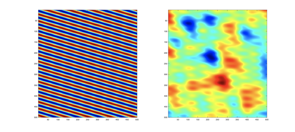
If Hiro’s snow in his VR headset is caused by laser speckle, then the seemingly random pattern is composed of amplitudes and phases that vary spatially and temporally.  There are many ways to make computer-generated versions of speckle.  One of the simplest is to just add together a lot of sinusoidal functions with varying orientations and periodicities.  This is a “Fourier” approach to speckle which views it as a random superposition of two-dimensional spatial frequencies.  An example is shown in Fig. 2 for one sinusoid which has been added to 20 others to generate the speckle pattern on the right.  There is still residual periodicity in the speckle for N = 20, but as N increases, the speckle pattern becomes strictly random, like noise. 

But if the sinusoids that are being added together link the periodicity with their amplitude through some functional relationship, then the final speckle can be analyze using a 2D Fourier transform to find its spatial frequency spectrum.  The functional form of this spectrum can tell a lot about the underlying processes of the speckle formation.  This is part of the information hidden inside snow.

(To watch animations of the figures in real time, See YouTube video.)

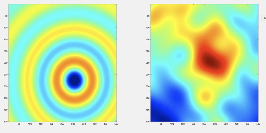
An alternative viewpoint to generating a laser speckle pattern thinks in terms of spatially-localized patches that add randomly together with random amplitudes and phases.  This is a space-domain view of speckle formation in contrast to the Fourier-space view of the previous construction.  Sinusoids are “global” extending spatially without bound. The underlying spatially localized functions can be almost any local function.  Gaussians spring to mind, but so do Airy functions, because they are common point-spread functions that participate in the formation of images through lenses.  The example in Fig 3a shows one such Airy function, and in 3b for speckle generated from N = 20 Airy functions of varying amplitudes and phases and locations.

These two examples are complementary ways of generating speckle, where the 2D Fourier-domain approach is conjugate to the 2D space-domain approach.

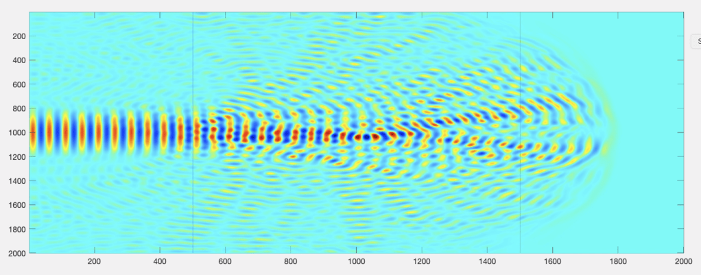
However, laser speckle is actually a 3D phenomenon, and the two-dimensional speckle patterns are just 2D cross sections intersecting a complex 3D pattern of light filaments.  To get a sense of how laser speckle is formed in a physical system, one can solve the propagation of a laser beam through a random optical medium.  In this way you can visualize the physical formation of the regions of brightness and darkness when the fragmented laser beam exits the random material. 

Coherent Patch

For a quantitative understanding of laser speckle, when 2D laser speckle is formed by an optical system, the central question is how big are the regions of brightness and darkness?  This is a question of spatial coherence, and one way to define spatial coherence is through the coherence area at the observation plane

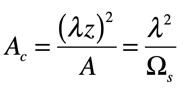
where A is the source emitting area, z is the distance to the observation plane, and Ω_s is the solid angle subtended by the source emitting area as seen from the observation point. This expression assumes that the angular spread of the light scattered from the illumination area is very broad. Larger distances and smaller emitting areas (pinholes in an optical diffuser or focused laser spots on a rough surface) produce larger coherence areas in the speckle pattern. For a Gaussian intensity distribution at the emission plane, the coherence area is

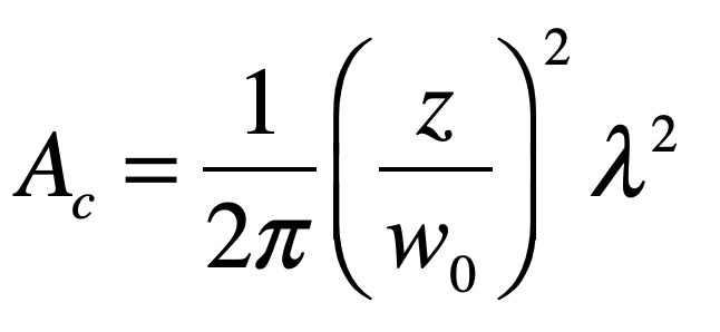
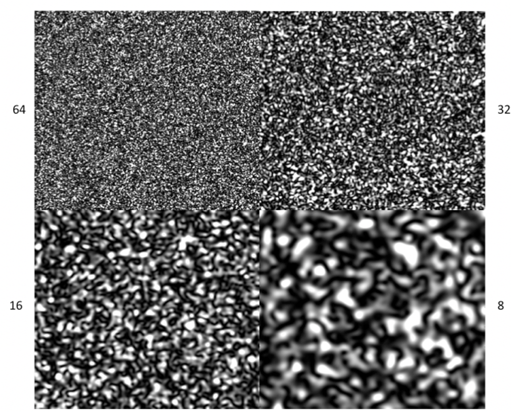
for beam waist w₀ at the emission plane.  To put some numbers to these parameters to give an intuitive sense of the size of speckle spots, assume a wavelength of 1 micron, a focused beam waist of 0.1 mm and a viewing distance of 1 meter.  This gives patches with a radius of about 2 millimeters.  Examples of laser speckle are shown in Fig. 5 for a variety of beam waist values w₀. 

Speckle Holograms

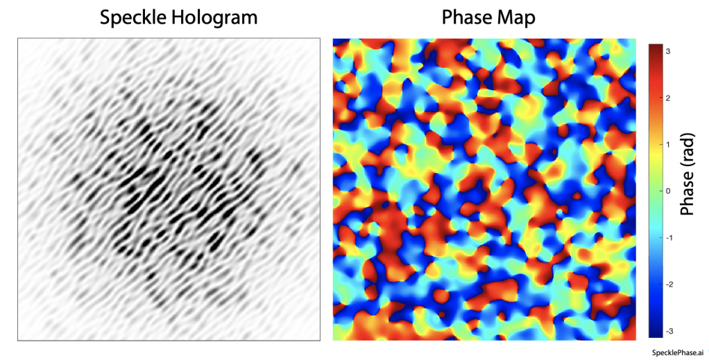
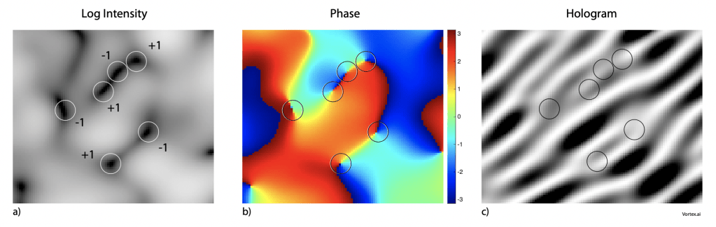
Associated with any intensity modulation must be a phase modulation through the Kramers-Kronig relations [2].  Phase cannot be detected directly in the speckle intensity pattern, but it can be measured by using interferometry.  One of the easiest interferometric techniques is holography in which a coherent plane wave is caused to intersect, at a small angle, a speckle pattern generated from the same laser source.  An example of a speckle hologram and its associated phase is shown in Fig. 6. The fringes of the hologram are formed when a plane reference wave interferes with the speckle field.  The fringes are not parallel because of the varying phase of the speckle field, but the average spatial frequency is still recognizable in Fig. 5a.  The associated phase map is shown in Fig. 5b.

Optical Vortex Physics

In the speckle intensity field, there are locations where the intensity vanishes, and the phase becomes undefined.  In the neighborhood of a singular point the phase wraps around it with a 2pi phase range.  Because of the wrapping phase such a singular point is called and optical vortex [3].  Vortices always come in pairs with opposite helicity (defined by the direction of the wrapping phase) with a line of neutral phase between them as shown in Fig. 7.  The helicity defines the topological charge of the vortex, and they can have topological charges larger than ±1 if the phase wraps multiple times.  In dynamic speckle these vortices are also dynamic and move with speeds related to the underlying dynamics of the scattering medium [4].  Vortices can annihilate if they have opposite helicity, and they can be created in pairs.  Studies of singular optics have merged with structured illumination [5] to create an active field of topological optics with applications in biological microscopy as well as material science.

---

References

[1] D. D. Nolte, Optical Interferometry for Biology and Medicine. (Springer, 2012)

[2] A. Mecozzi, C. Antonelli, and M. Shtaif, “Kramers-Kronig coherent receiver,” Optica, vol. 3, no. 11, pp. 1220-1227, Nov (2016)

[3] M. R. Dennis, R. P. King, B. Jack, K. O’Holleran, and M. J. Padgett, “Isolated optical vortex knots,” Nature Physics, vol. 6, no. 2, pp. 118-121, Feb (2010)

[4] S. J. Kirkpatrick, K. Khaksari, D. Thomas, and D. D. Duncan, “Optical vortex behavior in dynamic speckle fields,” Journal of Biomedical Optics, vol. 17, no. 5, May (2012), Art no. 050504

[5] H. Rubinsztein-Dunlop, A. Forbes, M. V. Berry, M. R. Dennis, D. L. Andrews, M. Mansuripur, C. Denz, C. Alpmann, P. Banzer, T. Bauer, E. Karimi, L. Marrucci, M. Padgett, M. Ritsch-Marte, N. M. Litchinitser, N. P. Bigelow, C. Rosales-Guzman, A. Belmonte, J. P. Torres, T. W. Neely, M. Baker, R. Gordon, A. B. Stilgoe, J. Romero, A. G. White, R. Fickler, A. E. Willner, G. D. Xie, B. McMorran, and A. M. Weiner, “Roadmap on structured light,” Journal of Optics, vol. 19, no. 1, Jan (2017), Art no. 013001