I often joke with my students in class that the reason I went into physics is because I have a bad memory. In biology you need to memorize a thousand things, but in physics you only need to memorize 10 things … and you derive everything else!
Of course, the first question they ask me is “What are those 10 things?”.
That’s a hard question to answer, and every physics professor probably has a different set of 10 things. Obviously, energy conservation would be first on the list, followed by other conservation laws for various types of momentum. Inverse-square laws probably come next. But then what? What do you need to memorize to be most useful when you are working out physics problems on the back of an envelope, when your phone is dead, and you have no access to your laptop or books?
One of my favorites is the Virial Theorem because it rears its head over and over again, whether you are working on problems in statistical mechanics, orbital mechanics or quantum mechanics.
The Virial Theorem
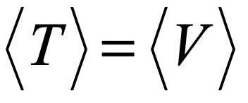
The Virial Theorem makes a simple statement about the balance between kinetic energy and potential energy (in a conservative mechanical system). It summarizes in a single form many different-looking special cases we learn about in physics. For instance, everyone learns early in their first mechanics course that the average kinetic energy <T> of a mass on a spring is equal to the average potential energy <V>. But this seems different than the problem of a circular orbit in gravitation or electrostatics where the average kinetic energy is equal to half the average potential energy, but with the opposite sign.
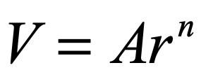
Yet there is a unity to these two—it is the Virial Theorem:
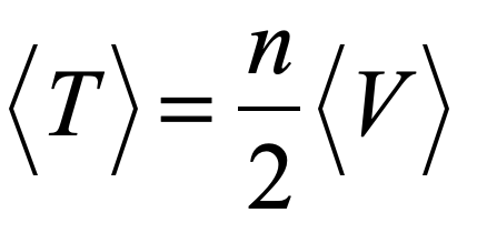
for cases where the potential energy V has power law dependence V ≈ rn. The harmonic oscillator has n = 2, leading to the well-known equality between average kinetic and potential energy as
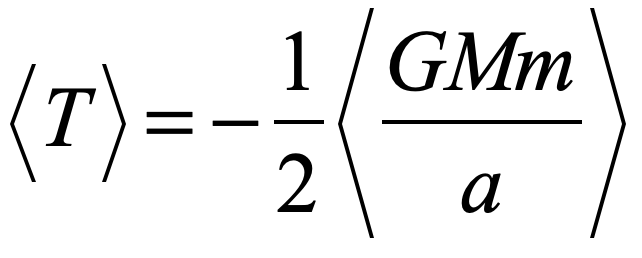
The inverse square force law has a potential that varies with n = -1, leading to the flip in sign. For instance, for a circular orbit in gravitation, it looks like
and in electrostatics it looks like
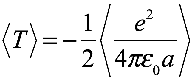
where a is the radius of the orbit.
Yet orbital mechanics is hardly the only place where the Virial Theorem pops up. It began its life with statistical mechanics.
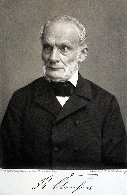
Rudolph Clausius and his Virial Theorem
The pantheon of physics is a somewhat exclusive club. It lets in the likes of Galileo, Lagrange, Maxwell, Boltzmann, Einstein, Feynman and Hawking, but it excludes many worthy candidates, like Gilbert, Stevin, Maupertuis, du Chatelet, Arago, Clausius, Heaviside and Meitner all of whom had an outsized influence on the history of physics, but who often do not get their due. Of this later group, Rudolph Clausius stands above the others because he was an inventor of whole new worlds and whole new terminologies that permeate physics today.
Within the German Confederation dominated by Prussia in the mid 1800’s, Clausius was among the first wave of the “modern” physicists who emerged from new or reorganized German universities that integrated mathematics with practical topics. Carl Neumann at Königsberg, Carl Gauss and Max Weber at Göttingen, and Hermann von Helmholtz at Berlin were transforming physics from a science focused on pure mechanics and astronomy to one focused on materials and their associated phenomena, applying mathematics to these practical problems.
Clausius was educated at Berlin under Heinrich Gustav Magnus beginning in 1840, and he completed his doctorate at the University of Halle in 1847. His doctoral thesis on light scattering in the atmosphere represented an early attempt at treating statistical fluctuations. Though his initial approach was naïve, it helped orient Clausius to physics problems of statistical ensembles and especially to gases. The sophistication of his physics matured rapidly and already in 1850 he published his famous paper Über die bewegende Kraft der Wärme, und die Gesetze, welche sich daraus für die Wärmelehre selbst ableiten lassen (About the moving power of heat and the laws that can be derived from it for the theory of heat itself).
This was the fundamental paper that overturned the archaic theory of caloric, which had assumed that heat was a form of conserved quantity. Clausius proved that this was not true, and he introduced what are today called the first and second laws of thermodynamics. This early paper was one in which he was still striving to simplify thermodynamics, and his second law was mostly a qualitative statement that heat flows from higher temperatures to lower. He refined the second law four years later in 1854 with Über eine veranderte Form des zweiten Hauptsatzes der mechanischen Wärmetheorie (On a modified form of the second law of the mechanical theory of heat). He gave his concept the name Entropy in 1865 from the Greek word τροπη (transformation or change) with a prefix similar to Energy.
Clausius was one of the first to consider the kinetic theory of heat where heat was understood as the average kinetic energy of the atoms or molecules that comprised the gas. He published his seminal work on the topic in 1857 expanding on earlier work by Augustus Krönig. Maxwell, in turn, expanded on Clausius in 1860 by introducing probability distributions. By 1870, Clausius was fully immersed in the kinetic theory as he was searching for mechanical proofs of the second law of thermodynamics. Along the way, he discovered a quantity based on action-reaction pairs of forces that was related to the kinetic energy.
At that time, kinetic energy was often called vis viva, meaning “living force”. The singular of force (vis) had a plural (virias), so Clausius—always happy to coin new words—called the action-reaction pairs of forces the virial, and hence he proved the Virial Theorem.
The argument is relatively simple. Consider the action of a single molecule of the gas subject to a force F that is applied reciprocally from another molecule. Also, for simplicity consider only a single direction in the gas. The change of the action over time is given by the derivative
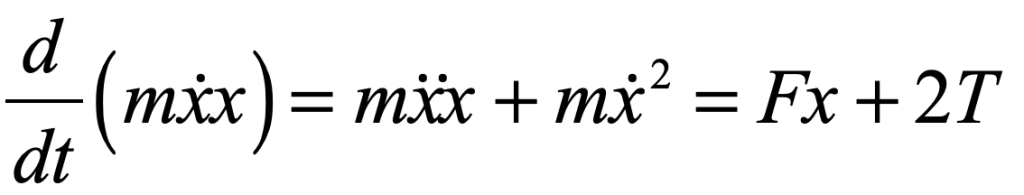
The average over all action-reaction pairs is
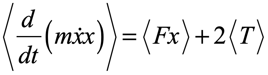
but by the reciprocal nature of action-reaction pairs, the left-hand side balances exactly to zero, giving
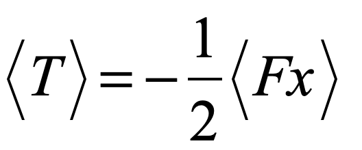
This expression is expanded to include the other directions and to all N bodies to yield the Virial Theorem
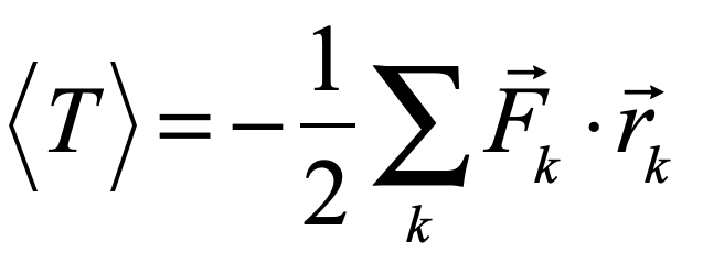
where the sum is over all molecules in the gas, and Clausius called the term on the right the Virial.
An important special case is when the force law derives from a power law
Then the Virial Theorem becomes (again in just one dimension)
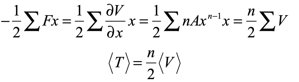
This is often the most useful form of the theorem. For a spring force, it leads to <T> = <V>. For gravitational or electrostatic orbits it is <T> = -1/2<V>.
The Virial in Astrophysics
Clausius originally developed the Virial Theorem for the kinetic theory of gases, but it has applications that go far beyond. It is already useful for simple orbital systems like masses interacting through central forces, and these can be scaled up to N-body systems like star clusters or galaxies.
Star clusters are groups of hundreds or thousands of stars that are gravitationally bound. Such a cluster may begin in a highly non-equilibrium configuration, but the mutual interactions among the stars causes a relaxation to an equilibrium configuration of positions and velocities. This process is known as Virialization. The time scale for virializaiton depends on the number of stars and on the initial configuration, such as whether there is a net angular momentum in the cluster.
A gravitational simulation of 700 stars is shown in Fig. 2. The stars are distributed uniformly with zero velocities. The cluster collapses under gravitational attraction, rebounds and approaches a steady state. The Virial Theorem applies at long times. The simulation assumed all motion was in the plane, and a regularization term was added to the gravitational potential to keep forces bounded.

The Virial in Quantum Physics
Quantum theory holds strong analogs to classical mechanics. For instance, the quantum commutation relations have strong similarities to Poisson Brackets. Similarly, the Virial in classical physics has a direct quantum analog.
Begin with the commutator between the Hamiltonian H and the action composed as the product of the position operator and the momentum operator XnPn
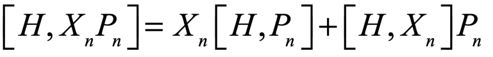
Expand the two commutators on the right to give
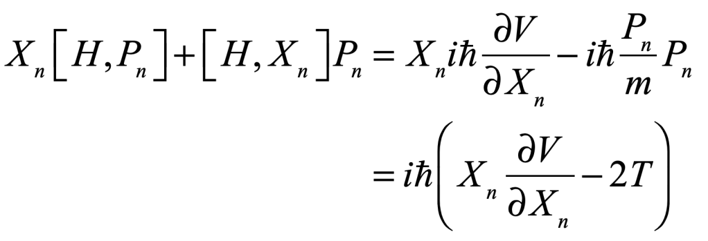
Now recognize that the commutator with the Hamiltonian is Ehrenfest’s Theorem on the time dependence of the operators
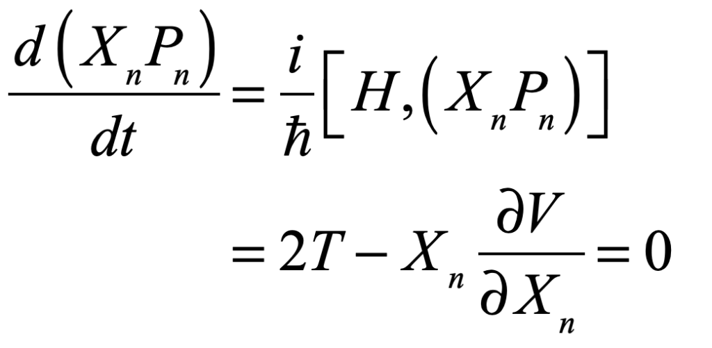
which equals zero when the system become stationary or steady state. All that remains is to take the expectation value of the equation (which can include many-body interactions as well)

which is the quantum form of the Virital Theorem which is identical to the classical form when the expectation value is replaced by the ensemble average.
For the hydrogen atom this is
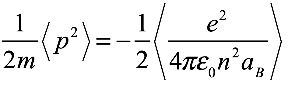
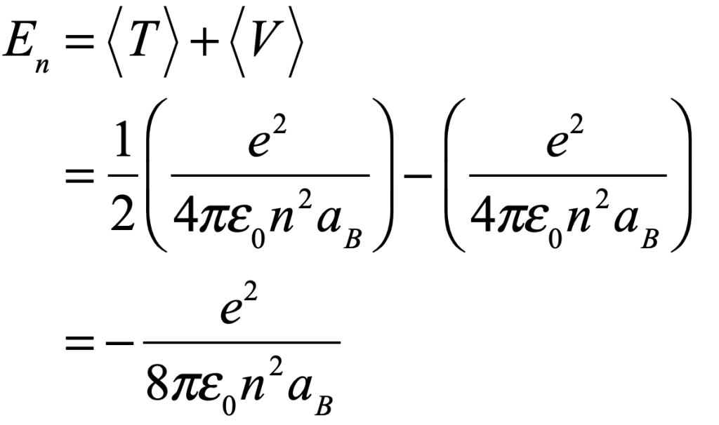
for principal quantum number n and Bohr radius aB. The quantum energy levels of the hydrogen atom are
By David D. Nolte, July 24, 2024
References
“Ueber die bewegende Kraft der Warme and die Gesetze welche sich daraus für die Warmelehre selbst ableiten lassen,” in Annalen der Physik, 79 (1850), 368–397, 500–524.
Über eine veranderte Form des zweiten Hauptsatzes der mechanischen Wärmetheorie, Annalen der Physik, 93 (1854), 481–506.
Ueber die Art der Bewegung, welche wir Warmenennen, Annalen der Physik, 100 (1857), 497–507.
Clausius, RJE (1870). “On a Mechanical Theorem Applicable to Heat”. Philosophical Magazine. Series 4. 40 (265): 122–127.
Matlab Code
function [y0,KE,Upoten,TotE] = Nbody(N,L)   %500, 100, 0

A = -1;        % Grav factor
eps = 1;        % 0.1
K = 0.00001;    %0.000025

format compact

mov_flag = 1;
if mov_flag == 1
    moviename = 'DrawNMovie';
    aviobj = VideoWriter(moviename,'MPEG-4');
    aviobj.FrameRate = 10;
    open(aviobj);
end

hh = colormap(jet);
%hh = colormap(gray);
rie = randintexc(255,255);       % Use this for random colors
%rie = 1:64;                     % Use this for sequential colors
for loop = 1:255
    h(loop,:) = hh(rie(loop),:);
end
figure(1)
fh = gcf;
clf;
set(gcf,'Color','White')
axis off

thet = 2*pi*rand(1,N);
rho = L*sqrt(rand(1,N));
X0 = rho.*cos(thet);
Y0 = rho.*sin(thet);

Vx0 = 0*Y0/L;   %1.5 for 500   2.0 for 700
Vy0 = -0*X0/L;
% X0 = L*2*(rand(1,N)-0.5);
% Y0 = L*2*(rand(1,N)-0.5);
% Vx0 = 0.5*sign(Y0);
% Vy0 = -0.5*sign(X0);
% Vx0 = zeros(1,N);
% Vy0 = zeros(1,N);

for nloop = 1:N
    y0(nloop) = X0(nloop);
    y0(nloop+N) = Y0(nloop);
    y0(nloop+2*N) = Vx0(nloop);
    y0(nloop+3*N) = Vy0(nloop);
end

T = 300;  %500
xp = zeros(1,N); yp = zeros(1,N);

for tloop = 1:T
    tloop

    delt = 0.005;
    tspan = [0 loop*delt];
    opts = odeset('RelTol',1e-2,'AbsTol',1e-5);
    [t,y] = ode45(@f5,tspan,y0,opts);

    %%%%%%%%% Plot Final Positions

    [szt,szy] = size(y);

    % Set nodes
    ind = 0; xpold = xp; ypold = yp;
    for nloop = 1:N
        ind = ind+1;
        xp(ind) = y(szt,ind+N);
        yp(ind) = y(szt,ind);
    end
    delxp = xp - xpold;
    delyp = yp - ypold;
    maxdelx = max(abs(delxp));
    maxdely = max(abs(delyp));
    maxdel = max(maxdelx,maxdely);

    rngx = max(xp) - min(xp);
    rngy = max(yp) - min(yp);
    maxrng = max(abs(rngx),abs(rngy));

    difepmx = maxdel/maxrng;

    crad = 2.5;
    subplot(1,2,1)
    gca;
    cla;

    % Draw nodes
    for nloop = 1:N
        rn = rand*63+1;
        colorval = ceil(64*nloop/N);

        rectangle('Position',[xp(nloop)-crad,yp(nloop)-crad,2*crad,2*crad],...
            'Curvature',[1,1],...
            'LineWidth',0.1,'LineStyle','-','FaceColor',h(colorval,:))

    end

    [syy,sxy] = size(y);
    y0(:) = y(syy,:);

    rnv = (2.0 + 2*tloop/T)*L;    % 2.0   1.5

    axis equal
    axis([-rnv rnv -rnv rnv])
    box on
    drawnow
    pause(0.01)

    KE = sum(y0(2*N+1:4*N).^2);

    Upot = 0;
    for nloop = 1:N
        for mloop = nloop+1:N
            dx = y0(nloop)-y0(mloop);
            dy = y0(nloop+N) - y0(mloop+N);
            dist = sqrt(dx^2+dy^2+eps^2);
            Upot = Upot + A/dist;
        end
    end

    Upoten = Upot;

    TotE = Upoten + KE;

    if tloop == 1
        TotE0 = TotE;
    end

    Upotent(tloop) = Upoten;
    KEn(tloop) = KE;
    TotEn(tloop) = TotE;

    xx = 1:tloop;
    subplot(1,2,2)
    plot(xx,KEn,xx,Upotent,xx,TotEn,'LineWidth',3)
    legend('KE','Upoten','TotE')
    axis([0 T -26000 22000])     % 3000 -6000 for 500   6000 -8000 for 700


    fh = figure(1);

    if mov_flag == 1
        frame = getframe(fh);
        writeVideo(aviobj,frame);
    end

end

if mov_flag == 1
    close(aviobj);
end

%%%%%%%%%%%%%%%%%%%%%%%%%%%%%%%%%%%%%%%%%%
    function yd = f5(t,y)

        for n1loop = 1:N

            posx = y(n1loop);
            posy = y(n1loop+N);
            momx = y(n1loop+2*N);
            momy = y(n1loop+3*N);

            tempcx = 0; tempcy = 0;

            for n2loop = 1:N
                if n2loop ~= n1loop
                    cposx = y(n2loop);
                    cposy = y(n2loop+N);
                    cmomx = y(n2loop+2*N);
                    cmomy = y(n2loop+3*N);

                    dis = sqrt((cposy-posy)^2 + (cposx-posx)^2 + eps^2);
                    CFx = 0.5*A*(posx-cposx)/dis^3 - 5e-5*momx/dis^4;
                    CFy = 0.5*A*(posy-cposy)/dis^3 - 5e-5*momy/dis^4;

                    tempcx = tempcx + CFx;
                    tempcy = tempcy + CFy;

                end
            end

            ypp(n1loop) = momx;
            ypp(n1loop+N) = momy;
            ypp(n1loop+2*N) = tempcx - K*posx;
            ypp(n1loop+3*N) = tempcy - K*posy;
        end

        yd=ypp';

    end     % end f5

end     % end Nbody