Intersystem crossing (ISC) for singlet-to-triplet transition and generation of singlet oxygen

A Story of Singlets and Triplets: Relativistic Biology

The tortoise and the hare.  The snail and the falcon.  The sloth and the cheetah.

Comparing the slowest animals to the fastest, the peregrine falcon wins in the air at 200 mph diving on a dove.  The cheetah wins on the ground at 75 mph running down dinner.  That’s fast!

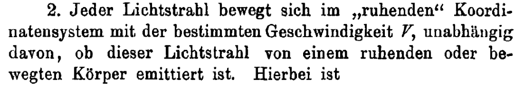
Einstein’s theory of relativity says that fast things behave differently than slow things.  So how fast do things need to move to see these effects?

The measure is the ratio of the speed of the object relative to the speed of light at 670 million miles per hour.  This ratio is called beta

The cheetah has β = 1×10⁻⁷, and the peregrine falcon has β = 4×10⁻⁷—which are less than one part in a million. 

And what about that snail?  At a speed of 0.003 mph it has β = 4×10-12 for a just few parts per trillion.

Yet relativistic physics is present in biology, despite these slow speeds, and they can help keep us alive.  How?

The Boon and Bane of Oxygen

All animal life on Earth needs oxygen to survive.  Oxygen is the energy storehouse that fuels mitochondria—the tiny batteries inside our cells that generate the energetic molecules that make us run.

Of all the elements, oxygen is second only to flourine as the most chemically reactive.  But fluorine is too one-dimensional to help much with life.  It needs only one extra electron to complete its outer-shell octet, leaving nothing in reserve to attach to much else.  Oxygen, on the other hand, needs two electrons to complete its outer shell, making it an easy bridge between two other atoms, usually carbons or hydrogens, and there you have it—organic chemistry is off and running.

Yet the same chemical reactivity that makes oxygen central to life also makes it corrosive to life.  When oxygen is not doing its part keeping things alive, it is tearing things apart.

The problem is reactive oxygen species, or ROS.  These are activated forms of oxygen that damage biological molecules, including DNA, putting wear and tear on (aging) the cellular machinery and introducing mutations into the genetic codes.  And one of the ROS is an active form of simple diatomic oxygen O2 — the very air we breathe.

The Saga of the Singlet and the Triplet

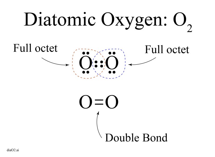
Diatomic oxygen is deceptively simple: two oxygen atoms, each two electrons short of a full shell, coming together to share two of each other’s electrons in a double bond, satisfying the closed shell octet for the outer valence electrons for this element.

Fig. 1 The Lewis diagram of the oxygen double bond.  Each oxygen shares two electrons with the other, filling the valence shell.

Bonds are based on energy levels, and the individual energy levels of the two separate oxygen atoms combine and shift as they form molecular orbitals (MO).  These orbitals are occupied by the 6 + 6 = 12 electrons of the diatomic molecule.  The first 10 electrons fill up the lower MOs until the last two go into the next highest state.  Here, for interesting reasons associated with how electrons interact with each other in confined spaces, the last two electrons both have the same orientation of their spins.  The total electron spin of the final full ground-state configuration of 12 electrons has S = 1. 

The unreactive triplet ground state molecular orbital diagram of diatomic oxygen (dioxygen). The two last electron spins are unpaired.
Fig. 2 Molecular orbital diagram for diatomic oxygen.  The 2s and 2p levels of the separated oxygen hybridize into new orbitals that are filled with 6 + 6 = 12 electrons.  The last two electron states have the same spin with a total spin S = 1.  This is the unreactive triplet ground state.

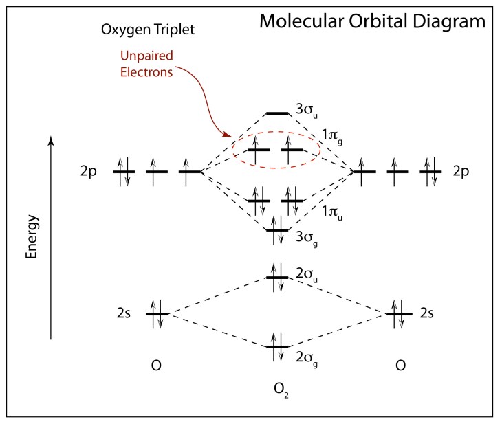
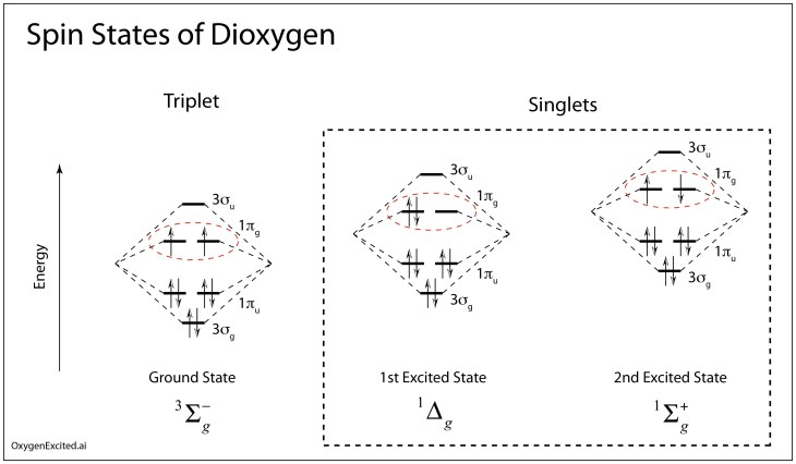
When a many-electron system has a spin S = 1, quantum mechanics prescribes that it has 2S+1 spin projections, so that the ground state of diatomic oxygen has three possible spin projections—known as a triplet.  But this is just for the lowest energy configuration of O2.

It is also possible to put both electrons into the final levels with opposite spins, giving S = 0.  This is known as the singlet, and there are two different ways these spins can be anti-aligned, creating two excited states.  The first excited state is about 1 eV in energy above the ground state, and the second excited state is about 0.7 eV higher than the first. 

The spin excited states of diatomic oxygen showing the pairing of spins to produce reactive singlet oxygen.
Fig. 3 Ground and excited states of O2.  The two singlet excited states have paired electron spins with a total spin of S = 0.  The ground state has S = 1.  The transitions between ground and excited states are “spin forbidden”.

Now we come the heart of our story.  It hinges on how reactive the different forms of O2 are, and how easily the singlet and the triplet can transform into each other.

Don’t Mix Your Spins

What happens if you mix hydrogen and oxygen in a 2:1 ratio in a plastic bag?

Nothing!  Unless you touch a match to it, and then it “pops” and creates water H2O.

Despite the thermodynamic instability of oxygen and hydrogen, the mixture is kinetically stable because it takes an additional input of energy to make the reaction go.  This is because oxygen at room temperature is almost exclusively in its ground state, the triplet state.  The triplet oxygen accepts electrons from other molecules, or atoms like hydrogen, but the local environment of organic molecules are almost exclusively in S = 0 states because of their stability. To accept two electrons from organic molecules requires spins to flip, which has an energy associated with the process, creating an energy barrier. This is known as the spin conservation rule of organic chemistry. Therefore, the reaction with the triplet is unlikely to go, unless you give it a hand with extra energy or a catalyst to get over the barrier.

However, this “spin blockade” that makes triplet (S = 1) oxygen unreactive (kinetically stable) is lifted in the case of singlet (S = 0) oxygen.  The singlet still accepts two electrons from other molecules, but these can be taken up easily by accepting electrons from the S = 0 organic molecules around it, conserving spin.  This makes singlet oxygen extremely reactive organically and hence is why it is an ROS. Singlet oxygen reacts with organic molecules, damaging them.

Despite the deleterious effects of singlet oxygen, it is produced as a side effect of lipids (fats) immersed in an oxygen environment. In a sense, fat slowly “burns”, creating reactive organic species that further react with lipids (primarily polyunsaturated fatty acids (PUFAs)), generating more ROS and creating a chain reaction. The chain reaction is terminated by the Russell mechanism that generates singlet oxygen as a byproduct.

Singlet oxygen, even though it is an excited state, cannot convert directly back to the benign triplet ground state for the same spin conservation reasons as organic chemistry. The singlet (S = 0) cannot emit a photon to get to its ground state triplet (S = 1) because photons cannot change the spin of the electrons in a transition. So once the singlet oxygen is formed, it can stick around and react chemically, eating up an organic molecule. Therefore, the oxygen environment, so necessary for our survival, is slowly killing us with oxydative stress. In response, mechanisms to de-excite singlet oxygen evolved, using organic molecules like carotenoids that are excellent physical quenchers of the singlet state.

But let’s flip the problem and ask what it takes to selectively harness singlet oxygen production to act as a targeted therapy that kills cancer cells—Enter Einstein’s theory of special relativity.

Relativistic Origins of Spin-Orbit Coupling

When I was a sophomore at Cornell University in the late 1970’s, I took the introductory class in electricity and magnetism. The text was an oddball thing from the Berkeley Physics Series authored by the Nobel Laureate, Edward Purcell, from Harvard.

Cover and front page of Purcell's E&M volume of the Berkeley Series.
Fig. 4 The cover and front page of my 1978 copy of Edward Purcell’s Berkeley Physics volume on Electricity and Magnetism.

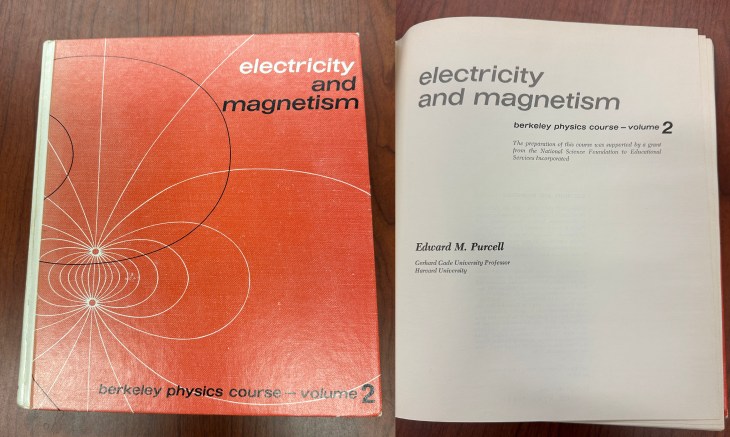
(The Berkeley Series was a set of 5 volumes to accompany a 5-semester introduction to physics. It was the brainchild of Charles Kittel from Berkeley and Philip Morrison from Cornell who, in 1961, were responding to the Sputnik crisis and the need to improve the teaching of physics in the West.)

Purcell’s book had the quirky misfortune to use Gaussian units based on centimeters and grams (cgs) instead of meters and kilograms (MKS). Physicists tend to like cgs units, especially in the teaching of electromagnetism, because it places electric fields and magnetic fields on equal footing. Unfortunately, it creates a weird set of units like “statvolts” and “statcoulombs” that are a nightmare to calculate with.

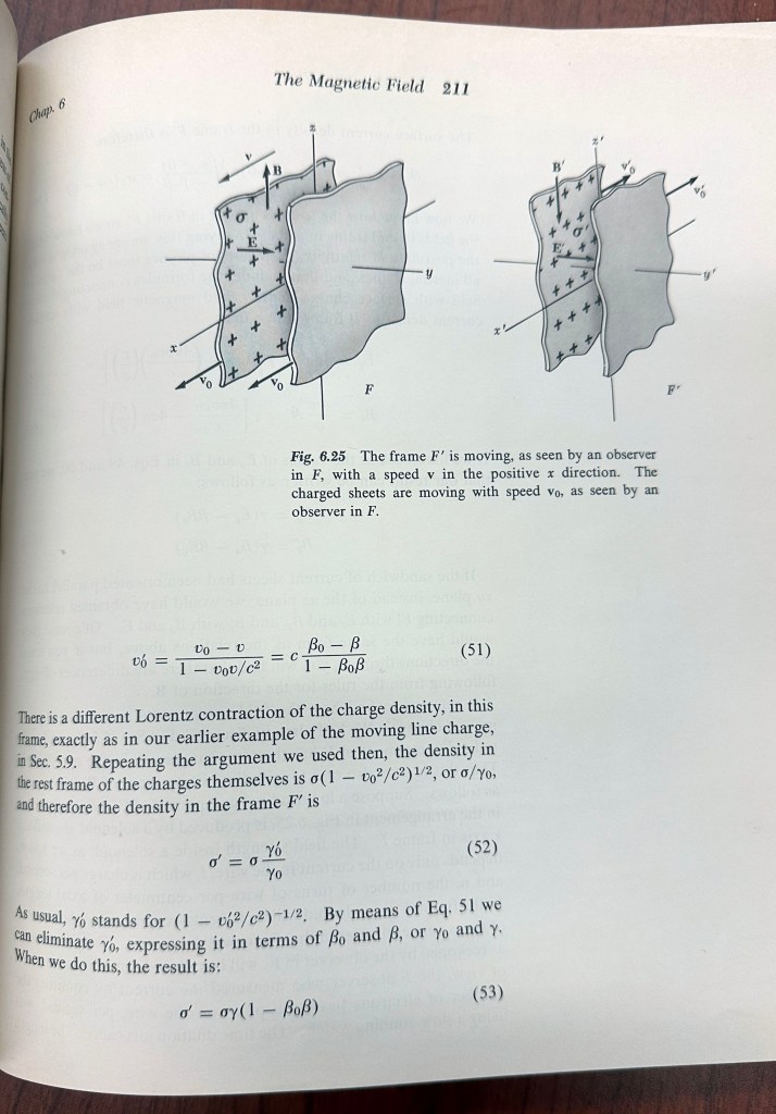
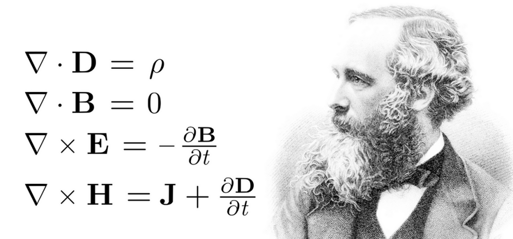
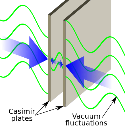
Nonetheless, Purcell’s book was revolutionary as a second-semester intro physics book, in that it used Special Relativity to explain the transformations between electric and magnetic fields. For instance, starting with the static electric field of a stationary parallel plate capacitor in one frame, Purcell showed how an observer moving relatively to the capacitor in a moving frame detects the electric field as expected, but also detects a slight magnetic field. As the speed of the observer increases, the strength of the magnetic field increases, becoming comparable to the electric field in strength as the relative frame speed approaches the speed of light.

In this way, there is one frame in which there is no magnetic field at all, and another frame in which there is a strong magnetic field. The only difference is the point of view—yet the consequences are profound, especially when the quantum spin of an electron is involved.

Conversion of E fields to B fields through relativistically moving frames
Fig. 5 Purcell’s use of a parallel plate capacitor in his demonstration of the origin of magnetic fields from electric fields in relatively moving frames.

The spin of the electron is like a tiny magnet, and if the spin is in an external magnetic field, it feels a torque as well as an interaction energy. The torque makes it precess, and the interaction energy shifts its energy levels depending on the orientation of the spin to the field.

When an electron is in a quantum orbital around a stationary nucleus, attracted by the electric field of the nucleus, it would seem that there is no magnetic field for the spin to interact with, which indeed is true if the electron has no angular momentum. But if the electron orbital does have angular momentum with a non-zero expectation value for its velocity, then this moving electron does experience a magnetic field—the electron is moving relative to the electric field of the nucleus, and special relativity dictates that it experiences a magnetic field. The resulting magnetic field interacts with the magnetic moment of the electron and shifts its energy a tiny amount.

Spin-orbit coupling and spin-forbidden transitions. Spin-orbit mixes singlet and triplet spin states.
Fig. 6 Transitions to the singlet excited state are allowed but to the triplet state are spin-forbidden. The spin-orbit coupling mixes the spin states, giving a little triplet character to the singlet and vice versa

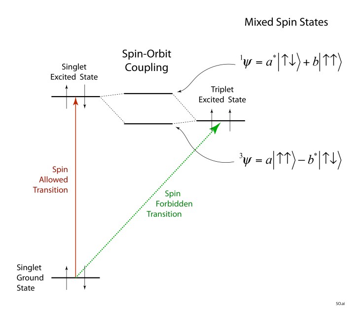
This is called the spin-orbit interaction and leads to the fine structure of the electron energy levels in atoms and molecules. More importantly for our story of Singlets and Triplets, the slight shift in energy also mixes the spin states. Quantum mechanical superposition of states mixes in a little S = 0 into the triplet excited state and a little S = 1 into the singlet ground state, and the transition is no longer strictly spin forbidden. The spin-orbit effect is relatively small in oxygen, contributing little to the quenching of singlet oxygen. But spin-orbit in other molecules, especially optical dyes that absorb light, can be used to generate singlet oxygen as a potent way to kill cancer cells.

Spin-Orbit and Photodynamic Cancer Therapy

The physics of light propagation through living tissue is a fascinating topic. Light is easily transported through tissue through multiple scattering. This is why your whole hand glows red when you cover a flashlight at night. The photons bounce around but are not easily absorbed. This surprising translucence of tissue can be used to help treat cancer.

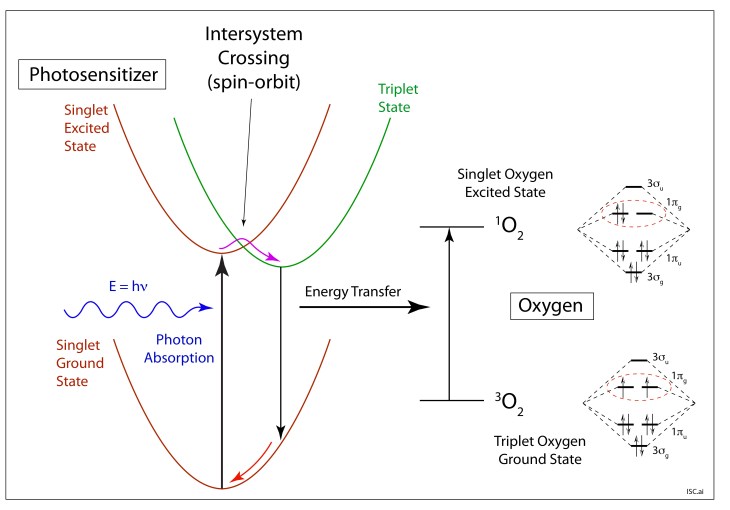
Photodynamic cancer therapy uses photosensitizer molecules, typically organic dyes, that absorb light, transforming the molecule from a single ground state to a singlet excited state (spin-allowed transition). Although singlet-to-triplet conversion is spin-forbidden, the spin-orbit coupling slightly mixes the spin states which allows a transformation known as intersystem crossing (ISC). The excited singlet crosses over (usually through a vibrational state associated with thermal energy) to an excited triplet state of the photosensitizer molecule. Oxygen triplet molecules, that are always prevalent in tissue, collide with the triplet photosensitizer—and they swap their energies in a spin-allowed transfer. The photosensitizer triplet returns to its singlet ground state, while the triplet oxygen converts to highly reactive singlet oxygen. The swap doesn’t change total spin, so it is allowed and fast, generating large amounts of reactive oxygen singlets.

Intersystem crossing (ISC) for singlet-to-triplet transition and generation of singlet oxygen
Fig. 7 Intersystem crossing diagram. A photosensitizer molecule in a singlet ground state absorbs a photon that creates a singlet excited state of the molecule. The spin-orbit mixing of spin states allows intersystem crossing (ISC) to generate a triplet excited state of the photosensitizer. This triplet can then exchange its energy with oxygen to create highly-reactive singlet oxygen.

In photodynamic therapy, the photosensitizer is taken up by the patient’s body, but the doctor only shines light around the tumor area, letting the light multiply-scatter through the tissue, exciting the photosensitizer and locally producing singlet oxygens that kill the local cancer cells. Other parts of the body remain in the dark and have none of the ill-effects that are so common for the conventional systemic cytotoxic anti-cancer drugs. This local treatment of the tumor using localized light can be much more benign to overall patient health while still delivering effective treatment to the tumor.

Photodynamic therapy has been approved by the FDA for some early stage cancers, and continuing research is expanding its applications. Because light transport through tissue is limited to about a centimeter, most of these applications are for “shallow” tumors that can be accessed by light through the skin or through internal surfaces (like the esophagus or colon).

Postscript: Relativistic Spin

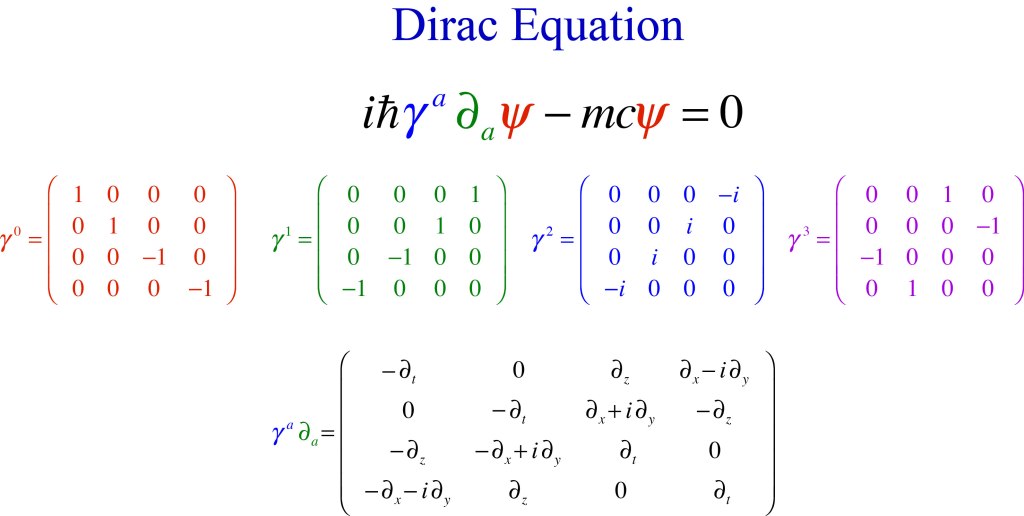
I can’t leave this story of relativistic biology without going into a final historical detail from the early days of relativistic quantum theory. When Uhlenbeck and Goudsmit first proposed in 1925 that the electron has spin, there were two immediate objections. First, Lorentz showed that in a semiclassical model of the spinning electron, the surface of the electron would be moving at 300 times the speed of light. The solution to this problem came three years later in 1928 with the relativistic quantum theory of Paul Dirac, which took an entirely different view of quantum versus classical physics. In quantum theory, there is no “radius of the electron” as there was in semiclassical theory.

The second objection was more serious. The original predictions from electron spin and the spin-orbit interaction in Bohr’s theory of the atom predicted a fine-structure splitting that was a factor of 2 times larger than observed experimentally. In 1926 Llewellyn Thomas showed that a relativistically precessing spin was in a non-inertial frame, requiring a continuous set of transformations from one instantaneously inertial frame to another. These continuously shifting transformations introduced a factor of 1/2 into the spin precession, exactly matching the experimental values. This effect is known as Thomas precession. Interestingly, the fully relativistic theory of Dirac in 1928 automatically incorporated this precession within the theory, so once again Dirac’s equation superseded the old quantum theory.

A Brief History of Nothing: The Physics of the Vacuum from Atomism to Higgs

It may be hard to get excited about nothing … unless nothing is the whole ball game. 

The only way we can really know what is, is by knowing what isn’t.  Nothing is the backdrop against which we measure something.  Experimentalists spend almost as much time doing control experiments, where nothing happens (or nothing is supposed to happen) as they spend measuring a phenomenon itself, the something.

Even the universe, full of so much something, came out of nothing during the Big Bang.  And today the energy density of nothing, so-called Dark Energy, is blowing our universe apart, propelling it ever faster to a bitter cold end.

So here is a brief history of nothing, tracing how we have understood what it is, where it came from, and where is it today.

With sturdy shoulders, space stands opposing all its weight to nothingness. Where space is, there is being.

Friedrich Nietzsche

40,000 BCE – Cosmic Origins

This is a human history, about how we homo sapiens try to understand the natural world around us, so the first step on a history of nothing is the Big Bang of human consciousness that occurred sometime between 100,000 – 40,000 years ago.  Some sort of collective phase transition happened in our thought process when we seem to have become aware of our own existence within the natural world.  This time frame coincides with the beginning of representational art and ritual burial.  This is also likely the time when human language skills reached their modern form, and when logical arguments–stories–first were told to explain our existence and origins. 

Roughly two origin stories emerged from this time.  One of these assumes that what is has always been, either continuously or cyclically.  Buddhism and Hinduism are part of this tradition as are many of the origin philosophies of Indigenous North Americans.  Another assumes that there was a beginning when everything came out of nothing.  Abrahamic faiths (Let there be light!) subscribe to this creatio ex nihilo.  What came before creation?  Nothing!

500 BCE – Leucippus and Democritus Atomism

The Greek philosopher Leucippus and his student Democritus, living around 500 BCE, were the first to lay out the atomic theory in which the elements of substance were indivisible atoms of matter, and between the atoms of matter was void.  The different materials around us were created by the different ways that these atoms collide and cluster together.  Plato later adhered to this theory, developing ideas along these lines in his Timeaus.

300 BCEAristotle Vacuum

Aristotle is famous for arguing, in his Physics Book IV, Section 8, that nature abhors a vacuum (horror vacui) because any void would be immediately filled by the imposing matter surrounding it.  He also argued more philosophically that nothing, by definition, cannot exist.

1644 – Rene Descartes Vortex Theory

Fast forward a millennia and a half, and theories of existence were finally achieving a level of sophistication that can be called “scientific”.  Rene Descartes followed Aristotle’s views of the vacuum, but he extended it to the vacuum of space, filling it with an incompressible fluid in his Principles of Philosophy (1644).  Just like water, laminar motion can only occur by shear, leading to vortices.  Descartes was a better philosopher than mathematician, so it took Christian Huygens to apply mathematics to vortex motion to “explain” the gravitational effects of the solar system.

Rene Descartes, Vortex Theory, 1644. Image Credit

1654 – Otto von Guericke Vacuum Pump

Otto von Guericke is one of those hidden gems of the history of science, a person who almost no-one remembers today, but who was far in advance of his own day.  He was a powerful politician, holding the position of Burgomeister of the city of Magdeburg for more than 30 years, helping to rebuild it after it was sacked during the Thirty Years War.  He was also a diplomat, playing a key role in the reorientation of power within the Holy Roman Empire.  How he had free time is anyone’s guess, but he used it to pursue scientific interests that spanned from electrostatics to his invention of the vacuum pump.

With a succession of vacuum pumps, each better than the last, von Geuricke was like a kid in a toy factory, pumping the air out of anything he could find.  In the process, he showed that a vacuum would extinguish a flame and could raise water in a tube.

The Magdeburg Experiment. Image Credit

His most famous demonstration was, of course, the Magdeburg sphere demonstration.  In 1657 he fabricated two 20-inch hemispheres that he attached together with a vacuum seal and used his vacuum pump to evacuate the air from inside.  He then attached chains from the hemispheres to a team of eight horses on each side, for a total of 16 horses, who were unable to separate the spheres.  This dramatically demonstrated that air exerts a force on surfaces, and that Aristotle and Descartes were wrong—nature did allow a vacuum!

1667 – Isaac Newton Action at a Distance

When it came to the vacuum, Newton was agnostic.  His universal theory of gravitation posited action at a distance, but the intervening medium played no direct role.

Nothing comes from nothing, Nothing ever could.

Rogers and Hammerstein, The Sound of Music

This would seem to say that Newton had nothing to say about the vacuum, but his other major work, his Optiks, established particles as the elements of light rays.  Such light particles travelled easily through vacuum, so the particle theory of light came down on the empty side of space.

Statue of Isaac Newton by Sir Eduardo Paolozzi based on a painting by William Blake. Image Credit

1821 – Augustin Fresnel Luminiferous Aether

Today, we tend to think of Thomas Young as the chief proponent for the wave nature of light, going against the towering reputation of his own countryman Newton, and his courage and insights are admirable.  But it was Augustin Fresnel who put mathematics to the theory.  It was also Fresnel, working with his friend Francois Arago, who established that light waves are purely transverse.

For these contributions, Fresnel stands as one of the greatest physicists of the 1800’s.  But his transverse light waves gave birth to one of the greatest red herrings of that century—the luminiferous aether.  The argument went something like this, “if light is waves, then just as sound is oscillations of air, light must be oscillations of some medium that supports it – the luminiferous aether.”  Arago searched for effects of this aether in his astronomical observations, but he didn’t see it, and Fresnel developed a theory of “partial aether drag” to account for Arago’s null measurement.  Hippolyte Fizeau later confirmed the Fresnel “drag coefficient” in his famous measurement of the speed of light in moving water.  (For the full story of Arago, Fresnel and Fizeau, see Chapter 2 of “Interference”. [1])

But the transverse character of light also required that this unknown medium must have some stiffness to it, like solids that support transverse elastic waves.  This launched almost a century of alternative ideas of the aether that drew in such stellar actors as George Green, George Stokes and Augustin Cauchy with theories spanning from complete aether drag to zero aether drag with Fresnel’s partial aether drag somewhere in the middle.

1849 – Michael Faraday Field Theory

Micheal Faraday was one of the most intuitive physicists of the 1800’s. He worked by feel and mental images rather than by equations and proofs. He took nothing for granted, able to see what his experiments were telling him instead of looking only for what he expected.

This talent allowed him to see lines of force when he mapped out the magnetic field around a current-carrying wire. Physicists before him, including Ampere who developed a mathematical theory for the magnetic effects of a wire, thought only in terms of Newton’s action at a distance. All forces were central forces that acted in straight lines. Faraday’s experiments told him something different. The magnetic lines of force were circular, not straight. And they filled space. This realization led him to formulate his theory for the magnetic field.

Others at the time rejected this view, until William Thomson (the future Lord Kelvin) wrote a letter to Faraday in 1845 telling him that he had developed a mathematical theory for the field. He suggested that Faraday look for effects of fields on light, which Faraday found just one month later when he observed the rotation of the polarization of light when it propagated in a high-index material subject to a high magnetic field. This effect is now called Faraday Rotation and was one of the first experimental verifications of the direct effects of fields.

Nothing is more real than nothing.

Samuel Beckett

In 1949, Faraday stated his theory of fields in their strongest form, suggesting that fields in empty space were the repository of magnetic phenomena rather than magnets themselves [2]. He also proposed a theory of light in which the electric and magnetic fields induced each other in repeated succession without the need for a luminiferous aether.

1861 – James Clerk Maxwell Equations of Electromagnetism

James Clerk Maxwell pulled the various electric and magnetic phenomena together into a single grand theory, although the four succinct “Maxwell Equations” was condensed by Oliver Heaviside from Maxwell’s original 15 equations (written using Hamilton’s awkward quaternions) down to the 4 vector equations that we know and love today.

One of the most significant and most surprising thing to come out of Maxwell’s equations was the speed of electromagnetic waves that matched closely with the known speed of light, providing near certain proof that light was electromagnetic waves.

However, the propagation of electromagnetic waves in Maxwell’s theory did not rule out the existence of a supporting medium—the luminiferous aether.  It was still not clear that fields could exist in a pure vacuum but might still be like the stress fields in solids.

Late in his life, just before he died, Maxwell pointed out that no measurement of relative speed through the aether performed on a moving Earth could see deviations that were linear in the speed of the Earth but instead would be second order.  He considered that such second-order effects would be far to small ever to detect, but Albert Michelson had different ideas.

1887 – Albert Michelson Null Experiment

Albert Michelson was convinced of the existence of the luminiferous aether, and he was equally convinced that he could detect it.  In 1880, working in the basement of the Potsdam Observatory outside Berlin, he operated his first interferometer in a search for evidence of the motion of the Earth through the aether.  He had built the interferometer, what has come to be called a Michelson Interferometer, months earlier in the laboratory of Hermann von Helmholtz in the center of Berlin, but the footfalls of the horse carriages outside the building disturbed the measurements too much—Postdam was quieter. 

But he could find no difference in his interference fringes as he oriented the arms of his interferometer parallel and orthogonal to the Earth’s motion.  A simple calculation told him that his interferometer design should have been able to detect it—just barely—so the null experiment was a puzzle.

Seven years later, again in a basement (this time in a student dormitory at Western Reserve College in Cleveland, Ohio), Michelson repeated the experiment with an interferometer that was ten times more sensitive.  He did this in collaboration with Edward Morley.  But again, the results were null.  There was no difference in the interference fringes regardless of which way he oriented his interferometer.  Motion through the aether was undetectable.

(Michelson has a fascinating backstory, complete with firestorms (literally) and the Wild West and a moment when he was almost committed to an insane asylum against his will by a vengeful wife.  To read all about this, see Chapter 4: After the Gold Rush in my recent book Interference (Oxford, 2023)).

The Michelson Morley experiment did not create the crisis in physics that it is sometimes credited with.  They published their results, and the physics world took it in stride.  Voigt and Fitzgerald and Lorentz and Poincaré toyed with various ideas to explain it away, but there had already been so many different models, from complete drag to no drag, that a few more theories just added to the bunch.

But they all had their heads in a haze.  It took an unknown patent clerk in Switzerland to blow away the wisps and bring the problem into the crystal clear.

1905 – Albert Einstein Relativity

So much has been written about Albert Einstein’s “miracle year” of 1905 that it has lapsed into a form of physics mythology.  Looking back, it seems like his own personal Big Bang, springing forth out of the vacuum.  He published 5 papers that year, each one launching a new approach to physics on a bewildering breadth of problems from statistical mechanics to quantum physics, from electromagnetism to light … and of course, Special Relativity [3].

Whereas the others, Voigt and Fitzgerald and Lorentz and Poincaré, were trying to reconcile measurements of the speed of light in relative motion, Einstein just replaced all that musing with a simple postulate, his second postulate of relativity theory:

  2. Any ray of light moves in the “stationary” system of co-ordinates with the determined velocity c, whether the ray be emitted by a stationary or by a moving body. Hence …

Albert Einstein, Annalen der Physik, 1905

And the rest was just simple algebra—in complete agreement with Michelson’s null experiment, and with Fizeau’s measurement of the so-called Fresnel drag coefficient, while also leading to the famous E = mc2 and beyond.

There is no aether.  Electromagnetic waves are self-supporting in vacuum—changing electric fields induce changing magnetic fields that induce, in turn, changing electric fields—and so it goes. 

The vacuum is vacuum—nothing!  Except that it isn’t.  It is still full of things.

1931 – P. A. M Dirac Antimatter

The Dirac equation is the famous end-product of P. A. M. Dirac’s search for a relativistic form of the Schrödinger equation. It replaces the asymmetric use in Schrödinger’s form of a second spatial derivative and a first time derivative with Dirac’s form using only first derivatives that are compatible with relativistic transformations [4]. 

One of the immediate consequences of this equation is a solution that has negative energy. At first puzzling and hard to interpret [5], Dirac eventually hit on the amazing proposal that these negative energy states are real particles paired with ordinary particles. For instance, the negative energy state associated with the electron was an anti-electron, a particle with the same mass as the electron, but with positive charge. Furthermore, because the anti-electron has negative energy and the electron has positive energy, these two particles can annihilate and convert their mass energy into the energy of gamma rays. This audacious proposal was confirmed by the American physicist Carl Anderson who discovered the positron in 1932.

The existence of particles and anti-particles, combined with Heisenberg’s uncertainty principle, suggests that vacuum fluctuations can spontaneously produce electron-positron pairs that would then annihilate within a time related to the mass energy

Although this is an exceedingly short time (about 10-21 seconds), it means that the vacuum is not empty, but contains a frothing sea of particle-antiparticle pairs popping into and out of existence.

1938 – M. C. Escher Negative Space

Scientists are not the only ones who think about empty space. Artists, too, are deeply committed to a visual understanding of our world around us, and the uses of negative space in art dates back virtually to the first cave paintings. However, artists and art historians only talked explicitly in such terms since the 1930’s and 1940’s [6].  One of the best early examples of the interplay between positive and negative space was a print made by M. C. Escher in 1938 titled “Day and Night”.

M. C. Escher. Day and Night. Image Credit

1946 – Edward Purcell Modified Spontaneous Emission

In 1916 Einstein laid out the laws of photon emission and absorption using very simple arguments (his modus operandi) based on the principles of detailed balance. He discovered that light can be emitted either spontaneously or through stimulated emission (the basis of the laser) [7]. Once the nature of vacuum fluctuations was realized through the work of Dirac, spontaneous emission was understood more deeply as a form of stimulated emission caused by vacuum fluctuations. In the absence of vacuum fluctuations, spontaneous emission would be inhibited. Conversely, if vacuum fluctuations are enhanced, then spontaneous emission would be enhanced.

This effect was observed by Edward Purcell in 1946 through the observation of emission times of an atom in a RF cavity [8]. When the atomic transition was resonant with the cavity, spontaneous emission times were much faster. The Purcell enhancement factor is

where Q is the “Q” of the cavity, and V is the cavity volume. The physical basis of this effect is the modification of vacuum fluctuations by the cavity modes caused by interference effects. When cavity modes have constructive interference, then vacuum fluctuations are larger, and spontaneous emission is stimulated more quickly.

1948 – Hendrik Casimir Vacuum Force

Interference effects in a cavity affect the total energy of the system by excluding some modes which become inaccessible to vacuum fluctuations. This lowers the internal energy internal to a cavity relative to free space outside the cavity, resulting in a net “pressure” acting on the cavity. If two parallel plates are placed in close proximity, this would cause a force of attraction between them. The effect was predicted in 1948 by Hendrik Casimir [9], but it was not verified experimentally until 1997 by S. Lamoreaux at Yale University [10].

Two plates brought very close feel a pressure exerted by the higher vacuum energy density external to the cavity.

1949 – Shinichiro Tomonaga, Richard Feynman and Julian Schwinger QED

The physics of the vacuum in the years up to 1948 had been a hodge-podge of ad hoc theories that captured the qualitative aspects, and even some of the quantitative aspects of vacuum fluctuations, but a consistent theory was lacking until the work of Tomonaga in Japan, Feynman at Cornell and Schwinger at Harvard. Feynman and Schwinger both published their theory of quantum electrodynamics (QED) in 1949. They were actually scooped by Tomonaga, who had developed his theory earlier during WWII, but physics research in Japan had been cut off from the outside world. It was when Oppenheimer received a letter from Tomonaga in 1949 that the West became aware of his work. All three received the Nobel Prize for their work on QED in 1965. Precision tests of QED now make it one of the most accurately confirmed theories in physics.

Richard Feynman’s first “Feynman diagram”.

1964 – Peter Higgs and The Higgs

The Higgs particle, known as “The Higgs”, was the brain-child of Peter Higgs, Francois Englert and Gerald Guralnik in 1964. Higgs’ name became associated with the theory because of a response letter he wrote to an objection made about the theory. The Higg’s mechanism is spontaneous symmetry breaking in which a high-symmetry potential can lower its energy by distorting the field, arriving at a new minimum in the potential. This mechanism can allow the bosons that carry force to acquire mass (something the earlier Yang-Mills theory could not do). 

Spontaneous symmetry breaking is a ubiquitous phenomenon in physics. It occurs in the solid state when crystals can lower their total energy by slightly distorting from a high symmetry to a low symmetry. It occurs in superconductors in the formation of Cooper pairs that carry supercurrents. And here it occurs in the Higgs field as the mechanism to imbues particles with mass . 

Conceptual graph of a potential surface where the high symmetry potential is higher than when space is distorted to lower symmetry. Image Credit

The theory was mostly ignored for its first decade, but later became the core of theories of electroweak unification. The Large Hadron Collider (LHC) at Geneva was built to detect the boson, announced in 2012. Peter Higgs and Francois Englert were awarded the Nobel Prize in Physics in 2013, just one year after the discovery.

The Higgs field permeates all space, and distortions in this field around idealized massless point particles are observed as mass. In this way empty space becomes anything but.

1981 – Alan Guth Inflationary Big Bang

Problems arose in observational cosmology in the 1970’s when it was understood that parts of the observable universe that should have been causally disconnected were in thermal equilibrium. This could only be possible if the universe were much smaller near the very beginning. In January of 1981, Alan Guth, then at Cornell University, realized that a rapid expansion from an initial quantum fluctuation could be achieved if an initial “false vacuum” existed in a positive energy density state (negative vacuum pressure). Such a false vacuum could relax to the ordinary vacuum, causing a period of very rapid growth that Guth called “inflation”. Equilibrium would have been achieved prior to inflation, solving the observational problem.Therefore, the inflationary model posits a multiplicities of different types of “vacuum”, and once again, simple vacuum is not so simple.

Energy density as a function of a scalar variable. Quantum fluctuations create a “false vacuum” that can relax to “normal vacuum: by expanding rapidly. Image Credit

1998 – Saul Pearlmutter Dark Energy

Einstein didn’t make many mistakes, but in the early days of General Relativity he constructed a theoretical model of a “static” universe. A central parameter in Einstein’s model was something called the Cosmological Constant. By tuning it to balance gravitational collapse, he tuned the universe into a static Ithough unstable) state. But when Edwin Hubble showed that the universe was expanding, Einstein was proven incorrect. His Cosmological Constant was set to zero and was considered to be a rare blunder.

Fast forward to 1999, and the Supernova Cosmology Project, directed by Saul Pearlmutter, discovered that the expansion of the universe was accelerating. The simplest explanation was that Einstein had been right all along, or at least partially right, in that there was a non-zero Cosmological Constant. Not only is the universe not static, but it is literally blowing up. The physical origin of the Cosmological Constant is believed to be a form of energy density associated with the space of the universe. This “extra” energy density has been called “Dark Energy”, filling empty space.

The expanding size of the Universe. Image Credit

Bottom Line

The bottom line is that nothing, i.e., the vacuum, is far from nothing. It is filled with a froth of particles, and energy, and fields, and potentials, and broken symmetries, and negative pressures, and who knows what else as modern physics has been much ado about this so-called nothing, almost more than it has been about everything else.

References:

[1] David D. Nolte, Interference: The History of Optical Interferometry and the Scientists Who Tamed Light (Oxford University Press, 2023)

[2] L. Peirce Williams in “Faraday, Michael.” Complete Dictionary of Scientific Biography, vol. 4, Charles Scribner’s Sons, 2008, pp. 527-540.

[3] A. Einstein, “On the electrodynamics of moving bodies,” Annalen Der Physik 17, 891-921 (1905).

[4] Dirac, P. A. M. (1928). “The Quantum Theory of the Electron”. Proceedings of the Royal Society A: Mathematical, Physical and Engineering Sciences. 117 (778): 610–624.

[5] Dirac, P. A. M. (1930). “A Theory of Electrons and Protons”. Proceedings of the Royal Society A: Mathematical, Physical and Engineering Sciences. 126 (801): 360–365.

[6] Nikolai M Kasak, Physical Art: Action of positive and negative space, (Rome, 1947/48) [2d part rev. in 1955 and 1956].

[7] A. Einstein, “Strahlungs-Emission un -Absorption nach der Quantentheorie,” Verh. Deutsch. Phys. Ges. 18, 318 (1916).

[8] Purcell, E. M. (1946-06-01). “Proceedings of the American Physical Society: Spontaneous Emission Probabilities at Ratio Frequencies”. Physical Review. American Physical Society (APS). 69 (11–12): 681.

[9] Casimir, H. B. G. (1948). “On the attraction between two perfectly conducting plates”. Proc. Kon. Ned. Akad. Wet. 51: 793.

[10] Lamoreaux, S. K. (1997). “Demonstration of the Casimir Force in the 0.6 to 6 μm Range”. Physical Review Letters. 78 (1): 5–8.


Read more in Books by David Nolte at Oxford University Press