Orion’s Dog: The Serious Science of Sirius

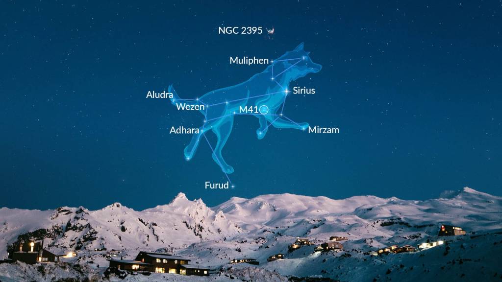
The constellation Orion strides high across the heavens on cold crisp winter nights in the North, followed at his heel by his constant companion, Canis Major, the Great Dog.  Blazing blue from the Dog’s proud chest is the star Sirius, the Dog Star, the brightest star in the night sky.  Although it is only the seventh closest star system to our sun, the other six systems host dimmer dwarf stars. Sirius, on the other hand, is a young bright star burning blue in the night.  It is an infant star, really, only as old as 5% the age of our sun, coming into being when Dinosaurs walked our planet.

The Sirius star system is a microcosm of mankind’s struggle to understand the Universe.  Because it is close and bright, it has become the de facto bench-test for new theories of astrophysics as well as for new astronomical imaging technologies.  It has played this role from the earliest days of history, when it was an element of religion rather than of science, down to the modern age as it continues to test and challenge new ideas about quantum matter and extreme physics.

Sirius Through the Ages

To the ancient Egyptians, Sirius was the star Sopdet, the welcome herald of the flooding of the Nile when it rose in the early morning sky of autumn.  The star was associated with Isis of the cow constellation Hathor (Canis Major) following closely behind Osiris (Orion).  The importance of the annual floods for the well-being of the ancient culture cannot be underestimated, and entire religions full of symbolic significance revolved around the heliacal rising of Sirius.

Fig. Canis Major.

To the Greeks, Sirius was always Sirius, although no one even as far back as Hesiod in the 7th century BC could recall where it got its name.  It was the dog star, as it was also to the Persians and the Hindus who called it Tishtrya and Tishya, respectively.  The loss of the initial “T” of these related Indo-European languages is a historical sound shift in relation to “S”, indicating that the name of the star dates back at least as far as the divergence of the Indo-European languages around the fourth millennium BC.  (Even more intriguing is the same association of Sirius with  dogs and wolves by the ancient Chinese and by Alaskan Innuits, as well as by many American Indian tribes, suggesting that the cultural significance of the star, if not its name, may have propagated across Asia and the Bering Strait as far back as the end of the last Ice Age.)  As the brightest star of the sky, this speaks to an enduring significance for Sirius, dating back to the beginning of human awareness of our place in nature.  No culture was unaware of this astronomical companion to the Sun and Moon and Planets.

The Greeks, too, saw Sirius as a harbinger, not for life-giving floods, but rather of the sweltering heat of late summer.  Homer, in the Iliad, famously wrote:

And aging Priam was the first to see him

sparkling on the plain, bright as that star

in autumn rising, whose unclouded rays

shine out amid a throng of stars at dusk—

the one they call Orion's dog, most brilliant,

yes, but baleful as a sign: it brings

great fever to frail men. So pure and bright

the bronze gear blazed upon him as he ran.

The Romans expanded on this view, describing “the dog days of summer”, which is a phrase that echoes till today as we wait for the coming coolness of autumn days.

The Heavens Move

The irony of the Copernican system of the universe, when it was proposed in 1543 by Nicolaus Copernicus, is that it took stars that moved persistently through the heavens and fixed them in the sky, unmovable.  The “fixed stars” became the accepted norm for several centuries, until the peripatetic Edmund Halley (1656 – 1742) wondered if the stars really did not move.  From Newton’s new work on celestial dynamics (the famous Principia, which Halley generously paid out of his own pocket to have published not only because of his friendship with Newton, but because Halley believed it to be a monumental work that needed to be widely known), it was understood that gravitational effects would act on the stars and should cause them to move.

Fig. Halley’s Comet

In 1710 Halley began studying the accurate star-location records of Ptolemy from one and a half millennia earlier and compared  them with what he could see in the night sky.  He realized that the star Sirius had shifted in the sky by an angular distance equivalent to the diameter of the moon.  Other bright stars, like Arcturus and Procyon, also showed discrepancies from Ptolemy.  On the other hand, dimmer stars, that Halley reasoned were farther away, showed no discernible shifts in 1500 years.  At a time when stellar parallax, the apparent shift in star locations caused by the movement of the Earth, had not yet been detected, Halley had found an alternative way to get at least some ranked distances to the stars based on their proper motion through the universe.  Closer stars to the Earth would show larger angular displacements over 1500 years than stars farther away.  By being the closest bright star to Earth, Sirius had become a testbed for observations and theories of the motions of stars.  With the confidence of the confirmation of the nearness of Sirius to the Earth, Jacques Cassini claimed in 1714 to have measured the parallax of Sirius, but Halley refuted this claim in 1720.  Parallax would remain elusive for another hundred years to come.

The Sound of Sirius

Of all the discoveries that emerged from nineteenth century physics—Young’s fringes, Biot-Savart law, Fresnel lens, Carnot cycle, Faraday effect, Maxwell’s equations, Michelson interferometer—only one is heard daily—the Doppler effect [1].  Doppler’s name is invoked every time you turn on the evening news to watch Doppler weather radar.  Doppler’s effect is experienced as you wait by the side of the road for a car to pass by or a jet to fly overhead.  Einstein may have the most famous name in physics, but Doppler’s is certainly the most commonly used.   

Although experimental support for the acoustic Doppler effect accumulated quickly, corresponding demonstrations of the optical Doppler effect were slow to emerge.  The breakthrough in the optical Doppler effect was made by William Huggins (1824-1910).  Huggins was an early pioneer in astronomical spectroscopy and was famous for having discovered that some bright nebulae consist of atomic gases (planetary nebula in our own galaxy) while others (later recognized as distant galaxies) consist of unresolved emitting stars.  Huggins was intrigued by the possibility of using the optical Doppler effect to measure the speed of stars, and he corresponded with James Clerk Maxwell (1831-1879) to confirm the soundness of Doppler’s arguments, which Maxwell corroborated using his new electromagnetic theory.  With the resulting confidence, Huggins turned his attention to the brightest star in the heavens, Sirius, and on May 14, 1868, he read a paper to the Royal Society of London claiming an observation of Doppler shifts in the spectral lines of the star Sirius consistent with a speed of about 50 km/sec [2].
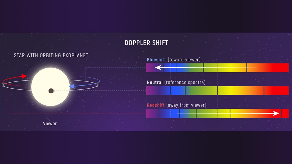
Fig. Doppler spectroscopy of stellar absorption lines caused by the relative motion of the star (in this illustration the orbiting exoplanet is causing the star to wobble.)

The importance of Huggins’ report on the Doppler effect from Sirius was more psychological than scientifically accurate, because it convinced the scientific community that the optical Doppler effect existed.  Around this time the German astronomer Hermann Carl Vogel (1841 – 1907) of the Potsdam Observatory began working with a new spectrograph designed by Johann Zöllner from Leipzig [3] to improve the measurements of the radial velocity of stars (the speed along the line of sight).  He was aware that the many values quoted by Huggins and others for stellar velocities were nearly the same as the uncertainties in their measurements.  Vogel installed photographic capabilities in the telescope and spectrograph at the Potsdam Observatory [4] in 1887 and began making observations of Doppler line shifts in stars through 1890.  He published an initial progress report in 1891, and then a definitive paper in 1892 that provided the first accurate stellar radial velocities [5].  Fifty years after Doppler read his paper to the Royal Bohemian Society of Science (in 1842 to a paltry crowd of only a few scientists), the Doppler effect had become an established workhorse of quantitative astrophysics. A laboratory demonstration of the optical Doppler effect was finally achieved in 1901 by Aristarkh Belopolsky (1854-1934), a Russian astronomer, by constructing a device with a narrow-linewidth light source and rapidly rotating mirrors [6].

White Dwarf

While measuring the position of Sirius to unprecedented precision, the German astronomer Friedrich Wilhelm Bessel (1784 – 1846) noticed a slow shift in its position.  (This is the same Bessel as “Bessel function” fame, although the functions were originally developed by Daniel Bernoulli and Bessel later generalized them.)  Bessel deduced that Sirius must have an unseen companion with an orbital of around 50 years.  This companion was discovered by accident in 1862 during a test run of a new lens manufactured by the Clark&Sons glass manufacturing company prior to delivery to Northwestern University in Chicago.  (The lens was originally ordered by the University of Mississippi in 1860, but after the Civil War broke out, the Massachusetts-based Clark company put it up for bid.  Harvard wanted it, but Northwestern got it.)  Sirius itself was redesignated Sirius A, while this new star was designated Sirius B (and sometimes called “The Pup”). 

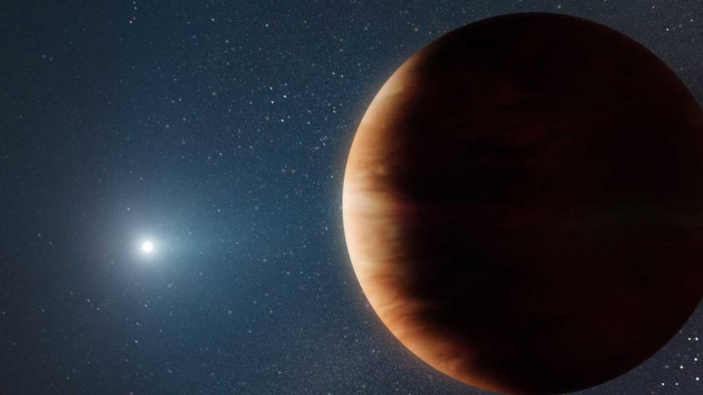
Fig. White dwarf and planet.

The Pup’s spectrum was measured in 1915 by Walter Adams (1876 – 1956) which put it in the newly-formed class of “white dwarf” stars that were very small but, unlike other types of dwarf stars, they had very hot (white) spectra.  The deflection of the orbit of Sirius A allowed its mass to be estimated at about one solar mass, which was normal for a dwarf star.  Furthermore, its brightness and surface temperature allowed its density to be estimated, but here an incredible number came out: the density of Sirius B was about 30,000 times greater than the density of the sun!  Astronomers at the time thought that this was impossible, and Arthur Eddington, who was the expert in star formation, called it “nonsense”.  This nonsense withstood all attempts to explain it for over a decade.

In 1926, R. H. Fowler (1889 – 1944) at Cambridge University in England applied the newly-developed theory of quantum mechanics and the Pauli exclusion principle to the problem of such ultra-dense matter.  He found that the Fermi sea of electrons provided a type of pressure, called degeneracy pressure, that counteracted the gravitational pressure that threatened to collapse the star under its own weight.  Several years later, Subrahmanyan Chandrasekhar calculated the upper limit for white dwarfs using relativistic effects and accurate density profiles and found that a white dwarf with a mass greater than about 1.5 times the mass of the sun would no longer be supported by the electron degeneracy pressure and would suffer gravitational collapse.  At the time, the question of what it would collapse to was unknown, although it was later understood that it would collapse to a neutron star.  Sirius B, at about one solar mass, is well within the stable range of white dwarfs.

But this was not the end of the story for Sirius B [7].  At around the time that Adams was measuring the spectrum of the white dwarf, Einstein was predicting that light emerging from a dense star would have its wavelengths gravitationally redshifted relative to its usual wavelength.  This was one of the three classic tests he proposed for his new theory of General Relativity.  (1 – The precession of the perihelion of Mercury. 2 – The deflection of light by gravity.  3 – The gravitational redshift of photons rising out of a gravity well.)  Adams announced in 1925 (after the deflection of light by gravity had been confirmed by Eddington in 1919) that he had measured the gravitational redshift.  Unfortunately, it was later surmised that he had not measured the gravitational effect but had actually measured Doppler-shifted spectra because of the rotational motion of the star.  The true gravitational redshift of Sirius B was finally measured in 1971, although the redshift of another white dwarf, 40 Eridani B, had already been measured in 1954.

Static Interference

The quantum nature of light is an elusive quality that requires second-order experiments of intensity fluctuations to elucidate them, rather than using average values of intensity.  But even in second-order experiments, the manifestations of quantum phenomenon are still subtle, as evidenced by an intense controversy that was launched by optical experiments performed in the 1950’s by a radio astronomer, Robert Hanbury Brown (1916 – 2002).  (For the full story, see Chapter 4 in my book Interference from Oxford (2023) [8]).

Hanbury Brown (he never went by his first name) was born in Aruvankandu, India, the son of a British army officer.  He never seemed destined for great things, receiving an unremarkable education that led to a degree in radio engineering from a technical college in 1935.  He hoped to get a PhD in radio technology, and he even received a scholarship to study at Imperial College in London, when he was urged by the rector of the university, Sir Henry Tizard, to give up his plans and join an effort to develop defensive radar against a growing threat from Nazi Germany as it aggressively rearmed after abandoning the punitive Versailles Treaty.  Hanbury Brown began the most exciting and unnerving five years of his life, right in the middle of the early development of radar defense, leading up to the crucial role it played in the Battle of Britain in 1940 and the Blitz from 1940 to 1941.  Partly due to the success of radar, Hitler halted night-time raids in the Spring of 1941, and England escaped invasion.

In 1949, fourteen years after he had originally planned to start his PhD, Hanbury Brown enrolled at the relatively ripe age of 33 at the University of Manchester.  Because of his background in radar, his faculty advisor told him to look into the new field of radio astronomy that was just getting started, and Manchester was a major player because it administrated the Jodrell Bank Observatory, which was one of the first and largest radio astronomy observatories in the World.  Hanbury Brown was soon applying all he had learned about radar transmitters and receivers to the new field, focusing particularly on aspects of radio interferometry after Martin Ryle (1918 – 1984) at Cambridge with Derek Vonberg (1921 – 2015) developed the first radio interferometer to measure the angular size of the sun [9] and of radio sources on the Sun’s surface that were related to sunspots [10].  Despite the success of their measurements, their small interferometer was unable to measure the size of other astronomical sources.  From Michelson’s formula for stellar interferometry, longer baselines between two separated receivers would be required to measure smaller angular sizes.  For his PhD project, Hanbury Brown was given the task of designing a radio interferometer to resolve the two strongest radio sources in the sky, Cygnus A and Cassiopeia A, whose angular sizes were unknown.  As he started the project, he was confronted with the problem of distributing a stable reference signal to receivers that might be very far apart, maybe even thousands of kilometers, a problem that had no easy solution. 

After grappling with this technical problem for months without success, late one night in 1949 Hanbury Brown had an epiphany [11], wondering what would happen if the two separate radio antennas measured only intensities rather than fields.  The intensity in a radio telescope fluctuates in time like random noise.  If that random noise were measured at two separated receivers while trained on a common source, would those noise patterns look the same?  After a few days considering this question, he convinced himself that the noise would indeed share common features, and the degree to which the two noise traces were similar should depend on the size of the source and the distance between the two receivers, just like Michelson’s fringe visibility.  But his arguments were back-of-the-envelope, so he set out to find someone with the mathematical skills to do it more rigorously.  He found Richard Twiss.

Richard Quentin Twiss (1920 – 2005), like Hanbury Brown, was born in India to British parents but had followed a more prestigious educational path, taking the Mathematical Tripos exam at Cambridge in 1941 and receiving his PhD from MIT in the United States in 1949.  He had just returned to England, joining the research division of the armed services located north of London, when he received a call from Hanbury Brown at the Jodrell Bank radio astronomy laboratory in Manchester.  Twiss travelled to meet Hanbury Brown in Manchester, who put him up in his flat in the neighboring town of Wilmslow.  The two set up the mathematical assumptions behind the new “intensity interferometer” and worked late into the night. When Hanbury Brown finally went to bed, Twiss was still figuring the numbers.  The next morning, the tall and lanky Twiss appeared in his silk dressing gown in the kitchen and told Hanbury Brown, “This idea of yours is no good, it doesn’t work”[12]—it would never be strong enough to detect the intensity from stars.  However, after haggling over the details of some of the integrals, Hanbury Brown, and then finally Twiss, became convinced that the effect was real.  Rather than fringe visibility, it was the correlation coefficient between two noise signals that would depend on the joint sizes of the source and receiver in a way that captured the same information as Michelson’s first-order fringe visibility.  But because no coherent reference wave was needed for interferometric mixing, this new approach could be carried out across very large baseline distances.

After demonstrating the effect on astronomical radio sources, Hanbury Brown and Twiss took the next obvious step: optical stellar intensity interferometry.  Their work had shown that photon noise correlations were analogous to Michelson fringe visibility, so the stellar intensity interferometer was expected to work similarly to the Michelson stellar interferometer—but with better stability over much longer baselines because it did not need a reference.  An additional advantage was the simple light collecting requirements.  Rather than needing a pair of massively expensive telescopes for high-resolution imaging, the intensity interferometer only needed to point two simple light collectors in a common direction.  For this purpose, and to save money, Hanbury Brown selected two of the largest army-surplus anti-aircraft searchlights that he could find left over from the London Blitz.  The lamps were removed and replaced with high-performance photomultipliers, and the units were installed on two train cars that could run along a railroad siding that crossed the Jodrell Bank grounds.
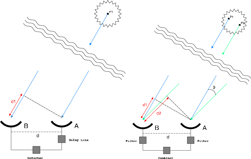
Fig. Stellar Interferometers: (Left) Michelson Stellar Field Interferometer. (Right) Hanbury Brown Twiss Stellar Intensity Interferometer.

The target of the first test of the intensity interferometer was Sirius, the Dog Star.  Sirius was chosen because it is the brightest star in the night sky and was close to Earth at 8.6 light years and hence would be expected to have a relatively large angular size.  The observations began at the start of winter in 1955, but the legendary English weather proved an obstacle.  In addition to endless weeks of cloud cover, on many nights dew formed on the reflecting mirrors, making it necessary to install heaters.  It took more than three months to make 60 operational attempts to accumulate a mere 18 hours of observations [13].  But it worked!  The angular size of Sirius was measured for the first time. It subtended an angle of approximately 6 milliarcseconds (mas), which was well within the expected range for such a main sequence blue star.  This angle is equivalent to observing a house on the Moon from the Earth.  No single non-interferometric telescope on Earth, or in Earth orbit, has that kind of resolution, even today.  Once again, Sirus was the testbed of a new observational technology.  Hanbury Brown and Twiss went on the measure the diameters of dozens of stars.

Adaptive Optics

Any undergraduate optics student can tell you that bigger telescopes have higher spatial resolution.  But this is only true up to a point.  When telescope diameters become not much bigger than about 10 inches, the images they form start to dance, caused by thermal fluctuations in the atmosphere.  Large telescopes can still get “lucky” at moments when the atmosphere is quiet, but this usually only happens for a fraction of a second before the fluctuation set in again.  This is the primary reason that the Hubble Space Telescope was placed in Earth orbit above the atmosphere, and why the James Webb Space Telescope is flying a million miles away from the Earth.  But that is not the end of Earth-based large telescoped.  The Very Large Telescope (VLT) has a primary diameter of 8 meters, and the Extremely Large Telescope (ELT), coming online soon, has an even bigger diameter of 40 meters.  How do these work under the atmospheric blanket?  The answer is adaptive optics.

Adaptive optics uses active feedback to measure the dancing images caused by the atmosphere and uses the information to control a flexible array of mirror elements to exactly cancel out the effects of the atmospheric fluctuations.  In the early days of adaptive-optics development, the applications were more military than astronomic, but advances made in imaging enemy satellites soon was released to the astronomers.  The first civilian demonstrations of adaptive optics were performed in 1977 when researchers at Bell Labs [14] and at the Space Sciences Lab at UC Berkeley [15] each made astronomical demonstrations of improved seeing of the star Sirius using adaptive optics.  The field developed rapidly after that, but once again Sirius had led the way.

Star Travel

The day is fast approaching when humans will begin thinking seriously of visiting nearby stars—not in person at first, but with unmanned spacecraft that can telemeter information back to Earth.  Although Sirius is not the closest star to Earth—it is 8.6 lightyears away while Alpha Centauri is almost twice as close at only 4.2 lightyears away—it may be the best target for an unmanned spacecraft.  The reason is its brightness. 

Stardrive technology is still in its infancy—most of it is still on drawing boards.  Therefore, the only “mature” technology we have today is light pressure on solar sails.  Within the next 50 years or so we will have the technical ability to launch a solar sail towards a nearby star and accelerate it to a good fraction of the speed of light.  The problem is decelerating the spaceship when it arrives at its destination, otherwise it will go zipping by with only a few seconds to make measurements after its long trek there.

Fig. NASA’s solar sail demonstrator unit (artist’s rendering).

A better idea is to let the star light push against the solar sail to decelerate it to orbital speed by the time it arrives.  That way, the spaceship can orbit the target star for years.  This is a possibility with Sirius.  Because it is so bright, its light can decelerate the spaceship even when it is originally moving at relativistic speeds. By one calculation, the trip to Sirius, including the deceleration and orbital insertion, should only take about 69 years [16].  That’s just one lifetime.  Signals could be beaming back from Sirius by as early as 2100—within the lifetimes of today’s children.


Footnotes

[1] The section is excerpted from D. D. Nolte, The Fall and Rise of the Doppler Effect, Physics Today (2020)

[2] W. Huggins, “Further observations on the spectra of some of the stars and nebulae, with an attempt to determine therefrom whether these bodies are moving towards or from the earth, also observations on the spectra of the sun and of comet II,” Philos. Trans. R. Soc. London vol. 158, pp. 529-564, 1868. The correct value is -5.5 km/sec approaching Earth.  Huggins got the magnitude and even the sign wrong.

[3] in Hearnshaw, The Analysis of Starlight (Cambridge University Press, 2014), pg. 89

[4] The Potsdam Observatory was where the American Albert Michelson built his first interferometer while studying with Helmholtz in Berlin.

[5] Vogel, H. C. Publik. der astrophysik. Observ. Potsdam 1: 1. (1892)

[6] A. Belopolsky, “On an apparatus for the laboratory demonstration of the Doppler-Fizeau principle,” Astrophysical Journal, vol. 13, pp. 15-24, Jan 1901.

[7] https://adsabs.harvard.edu/full/1980QJRAS..21..246H

[8] D. D. Nolte, Interference: The History of Optical Interferometry and the Scientists who Tamed Light (Oxford University Press, 2023)

[9] M. Ryle and D. D. Vonberg, “Solar Radiation on 175 Mc/sec,” Nature, vol. 158 (1946): pp. 339-340.; K. I. Kellermann and J. M. Moran, “The development of high-resolution imaging in radio astronomy,” Annual Review of Astronomy and Astrophysics, vol. 39, (2001): pp. 457-509.

[10] M. Ryle, ” Solar radio emissions and sunspots,” Nature, vol. 161, no. 4082 (1948): pp. 136-136.

[11] R. H. Brown, The intensity interferometer; its application to astronomy (London, New York, Taylor & Francis; Halsted Press, 1974).

[12] R. H. Brown, Boffin : A personal story of the early days of radar and radio astronomy (Adam Hilger, 1991), p. 106.

[13] R. H. Brown and R. Q. Twiss. ” Test of a new type of stellar interferometer on Sirius.” Nature 178, no. 4541 (1956): pp. 1046-1048.

[14] S. L. McCall, T. R. Brown, and A. Passner, “IMPROVED OPTICAL STELLAR IMAGE USING A REAL-TIME PHASE-CORRECTION SYSTEM – INITIAL RESULTS,” Astrophysical Journal, vol. 211, no. 2, pp. 463-468, (1977)

[15] A. Buffington, F. S. Crawford, R. A. Muller, and C. D. Orth, “1ST OBSERVATORY RESULTS WITH AN IMAGE-SHARPENING TELESCOPE,” Journal of the Optical Society of America, vol. 67, no. 3, pp. 304-305, 1977 (1977)

[16] https://www.newscientist.com/article/2128443-quickest-we-could-visit-another-star-is-69-years-heres-how/
New Book: Interference. The Scientists who Tamed Light

 Interference: The History of Optical Interferometry and the Scientists who Tamed Light, is published! It is available now at Oxford University Press and can be pre-ordered at Amazon and Barnes&Nobles to ship on Sept. 6.

The synopses of the first chapters can be found in my previous blog. Here are previews of the final chapters.

Chapter 6. Across the Universe: Exoplanets, Black Holes and Gravitational Waves

Stellar interferometry is opening new vistas of astronomy, exploring the wildest occupants of our universe, from colliding black holes half-way across the universe (LIGO) to images of neighboring black holes (EHT) to exoplanets near Earth that may harbor life.

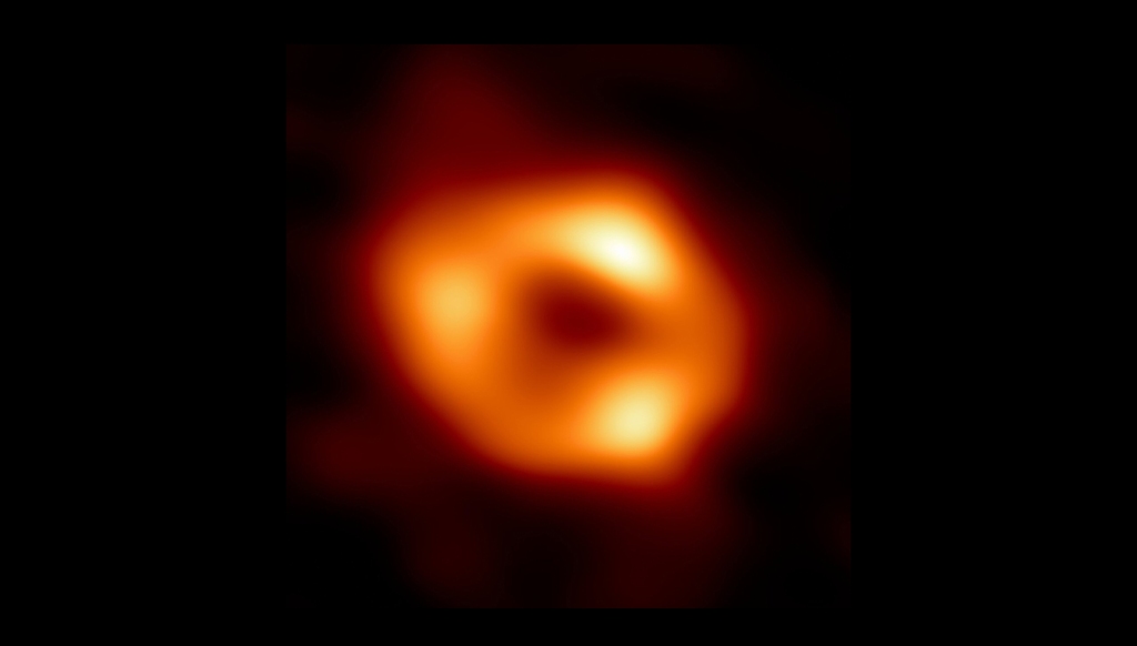
Image of the supermassive black hole in M87 from Event Horizon Telescope.

Across the Universe: Gravitational Waves, Black Holes and the Search for Exoplanets describes the latest discoveries of interferometry in astronomy including the use of nulling interferometry in the Very Large Telescope Interferometer (VLTI) to detect exoplanets orbiting distant stars.  The much larger Event Horizon Telescope (EHT) used long baseline interferometry and closure phase advanced by Roger Jenison to make the first image of a black hole.  The Laser Interferometric Gravitational Observatory (LIGO) represented a several-decade-long drive to detect the first gravitational waves first predicted by Albert Einstein a hundred years ago.

Chapter 7. Two Faces of Microscopy: Diffraction and Interference

From the astronomically large dimensions of outer space to the microscopically small dimensions of inner space, optical interference pushes the resolution limits of imaging.

Ernst Abbe. Image Credit.

Two Faces of Microscopy: Diffraction and Interference describes the development of microscopic principles starting with Joseph Fraunhofer and the principle of diffraction gratings that was later perfected by Henry Rowland for high-resolution spectroscopy.  The company of Carl Zeiss advanced microscope technology after enlisting the help of Ernst Abbe who formed a new theory of image formation based on light interference.  These ideas were extended by Fritz Zernike in the development of phase-contrast microscopy.  The ultimate resolution of microscopes, defined by Abbe and known as the Abbe resolution limit, turned out not to be a fundamental limit, but was surpassed by super-resolution microscopy using concepts of interference microscopy and structured illumination.

Chapter 8. Holographic Dreams of Princess Leia: Crossing Beams

The coherence of laser light is like a brilliant jewel that sparkles in the darkness, illuminating life, probing science and projecting holograms in virtual worlds.

Ted Maiman

Holographic Dreams of Princess Leia: Crossing Beams presents the history of holography, beginning with the original ideas of Denis Gabor who invented optical holography as a means to improve the resolution of electron microscopes.  Holography became mainstream after the demonstrations by Emmett Leith and Juris Upatnieks using lasers that were first demonstrated by Ted Maiman at Hughes Research Lab after suggestions by Charles Townes on the operating principles of the optical maser.  Dynamic holography takes place in crystals that exhibit the photorefractive effect that are useful for adaptive interferometry.  Holographic display technology is under development, using ideas of holography merged with light-field displays that were first developed by Gabriel Lippmann.

Chapter 9. Photon Interference: The Foundations of Quantum Communication and Computing

What is the image of one photon interfering? Better yet, what is the image of two photons interfering? The answer to this crucial question laid the foundation for quantum communication.

Leonard Mandel. Image Credit.

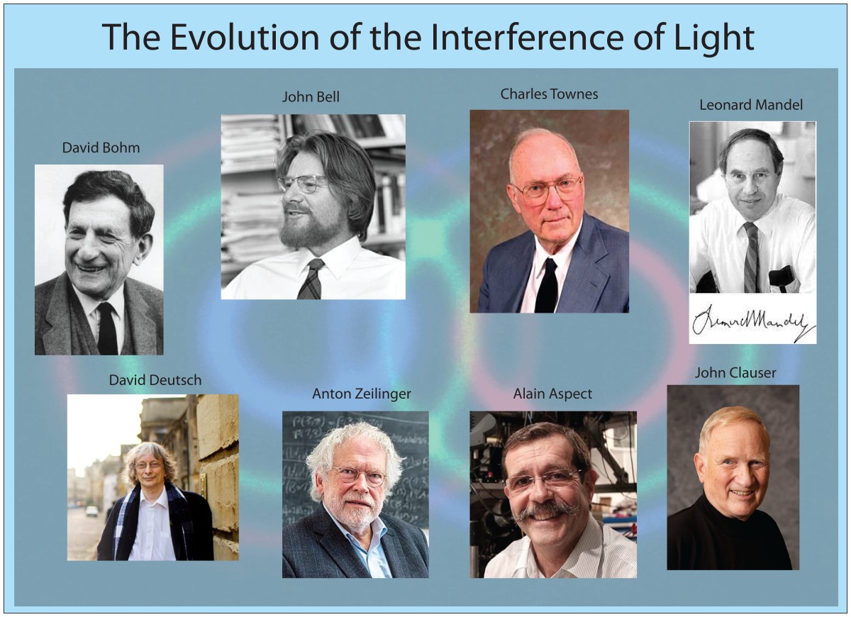
Photon Interference: The Foundations of Quantum Communication moves the story of interferometry into the quantum realm, beginning with the Einstein-Podolski-Rosen paradox and the principle of quantum entanglement that was refined by David Bohm who tried to banish uncertainty from quantum theory.  John Bell and John Clauser pushed the limits of what can be known from quantum measurement as Clauser tested Bell’s inequalities, confirming the fundamental nonlocal character of quantum systems.  Leonard Mandel pushed quantum interference into the single-photon regime, discovering two-photon interference fringes that illustrated deep concepts of quantum coherence.  Quantum communication began with quantum cryptography and developed into quantum teleportation that can provide the data bus of future quantum computers.

Chapter 10. The Quantum Advantage: Interferometric Computing

There is almost no technical advantage better than having exponential resources at hand. The exponential resources of quantum interference provide that advantage to quantum computing which is poised to usher in a new era of quantum information science and technology.

David Deutsch.

The Quantum Advantage: Interferometric Computing describes the development of quantum algorithms and quantum computing beginning with the first quantum algorithm invented by David Deutsch as a side effect of his attempt to prove the multiple world interpretation of quantum theory.  Peter Shor found a quantum algorithm that could factor the product of primes and that threatened all secure communications in the world.  Once the usefulness of quantum algorithms was recognized, quantum computing hardware ideas developed rapidly into quantum circuits supported by quantum logic gates.  The limitation of optical interactions, that hampered the development of controlled quantum gates, led to the proposal of linear optical quantum computing and boson sampling in a complex cascade of single-photon interferometers that has been used to demonstrate quantum supremacy, also known as quantum computational advantage, using photonic integrated circuits.


New from Oxford Press: Interference

A popular account of the trials and toils of the scientists and engineers who tamed light and used it to probe the universe.

Book Preview: Interference. The History of Optical Interferometry

This history of interferometry has many surprising back stories surrounding the scientists who discovered and explored one of the most important aspects of the physics of light—interference. From Thomas Young who first proposed the law of interference, and Augustin Fresnel and Francois Arago who explored its properties, to Albert Michelson, who went almost mad grappling with literal firestorms surrounding his work, these scientists overcame personal and professional obstacles on their quest to uncover light’s secrets. The book’s stories, told around the topic of optics, tells us something more general about human endeavor as scientists pursue science.

Interference: The History of Optical Interferometry and the Scientists who Tamed Light, was published Ag. 6 and is available at Oxford University Press and Amazon. Here is a brief preview of the frist several chapters:

Chapter 1. Thomas Young Polymath: The Law of Interference

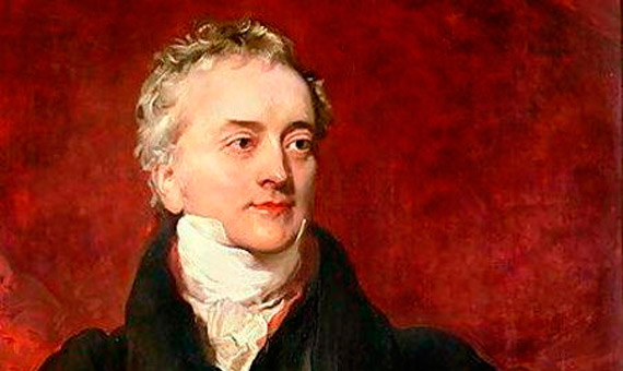
Thomas Young was the ultimate dabbler, his interests and explorations ranged far and wide, from ancient egyptology to naval engineering, from physiology of perception to the physics of sound and light. Yet unlike most dabblers who accomplish little, he made original and seminal contributions to all these fields. Some have called him the “Last Man Who Knew Everything”.

Thomas Young. The Law of Interference.

The chapter, Thomas Young Polymath: The Law of Interference, begins with the story of the invasion of Egypt in 1798 by Napoleon Bonaparte as the unlikely link among a set of epic discoveries that launched the modern science of light.  The story of interferometry passes from the Egyptian campaign and the discovery of the Rosetta Stone to Thomas Young.  Young was a polymath, known for his facility with languages that helped him decipher Egyptian hieroglyphics aided by the Rosetta Stone.  He was also a city doctor who advised the admiralty on the construction of ships, and he became England’s premier physicist at the beginning of the nineteenth century, building on the wave theory of Huygens, as he challenged Newton’s particles of light.  But his theory of the wave nature of light was controversial, attracting sharp criticism that would pass on the task of refuting Newton to a new generation of French optical physicists.

Chapter 2. The Fresnel Connection: Particles versus Waves

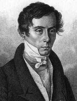
Augustin Fresnel was an intuitive genius whose talents were almost squandered on his job building roads and bridges in the backwaters of France until he was discovered and rescued by Francois Arago.

Augustin Fresnel. Image Credit.

The Fresnel Connection: Particles versus Waves describes the campaign of Arago and Fresnel to prove the wave nature of light based on Fresnel’s theory of interfering waves in diffraction.  Although the discovery of the polarization of light by Etienne Malus posed a stark challenge to the undulationists, the application of wave interference, with the superposition principle of Daniel Bernoulli, provided the theoretical framework for the ultimate success of the wave theory.  The final proof came through the dramatic demonstration of the Spot of Arago.

Chapter 3. At Light Speed: The Birth of Interferometry

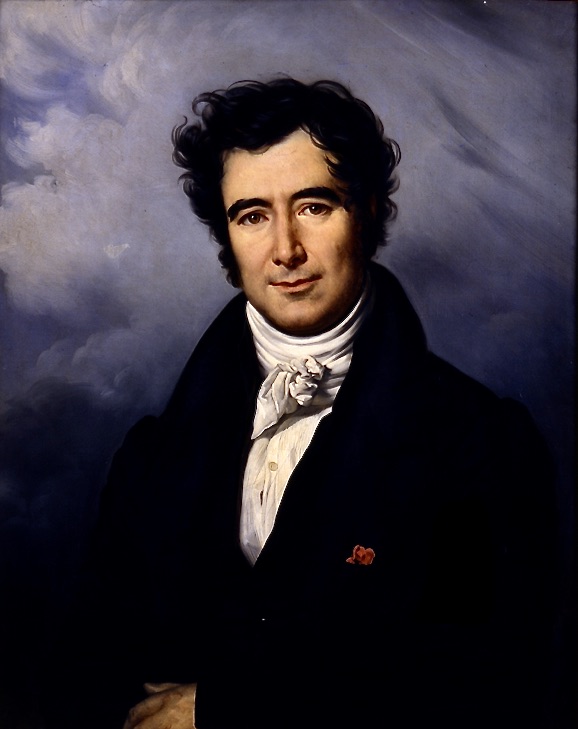
There is no question that Francois Arago was a swashbuckler. His life’s story reads like an adventure novel as he went from being marooned in hostile lands early in his career to becoming prime minister of France after the 1848 revolutions swept across Europe.

Francois Arago. Image Credit.

At Light Speed: The Birth of Interferometry tells how Arago attempted to use Snell’s Law to measure the effect of the Earth’s motion through space but found no effect, in contradiction to predictions using Newton’s particle theory of light.  Direct measurements of the speed of light were made by Hippolyte Fizeau and Leon Foucault who originally began as collaborators but had an epic falling-out that turned into an  intense competition.  Fizeau won priority for the first measurement, but Foucault surpassed him by using the Arago interferometer to measure the speed of light in air and water with increasing accuracy.  Jules Jamin later invented one of the first interferometric instruments for use as a refractometer.

Chapter 4. After the Gold Rush: The Trials of Albert Michelson

No name is more closely connected to interferometry than that of Albert Michelson. He succeeded, sometimes at great personal cost, in launching interferometric metrology as one of the most important tools used by scientists today.

Albert A. Michelson, 1907 Nobel Prize. Image Credit.

After the Gold Rush: The Trials of Albert Michelson tells the story of Michelson’s youth growing up in the gold fields of California before he was granted an extraordinary appointment to Annapolis by President Grant. Michelson invented his interferometer while visiting Hermann von Helmholtz in Berlin, Germany, as he sought to detect the motion of the Earth through the luminiferous ether, but no motion was detected. After returning to the States and a faculty position at Case University, he met Edward Morley, and the two continued the search for the Earth’s motion, concluding definitively its absence.  The Michelson interferometer launched a menagerie of interferometers (including the Fabry-Perot interferometer) that ushered in the golden age of interferometry.

Chapter 5. Stellar Interference: Measuring the Stars

Learning from his attempts to measure the speed of light through the ether, Michelson realized that the partial coherence of light from astronomical sources could be used to measure their sizes. His first measurements using the Michelson Stellar Interferometer launched a major subfield of astronomy that is one of the most active today.

R Hanbury Brown

Stellar Interference: Measuring the Stars brings the story of interferometry to the stars as Michelson proposed stellar interferometry, first demonstrated on the Galilean moons of Jupiter, followed by an application developed by Karl Schwarzschild for binary stars, and completed by Michelson with observations encouraged by George Hale on the star Betelgeuse.  However, the Michelson stellar interferometry had stability limitations that were overcome by Hanbury Brown and Richard Twiss who developed intensity interferometry based on the effect of photon bunching.  The ultimate resolution of telescopes was achieved after the development of adaptive optics that used interferometry to compensate for atmospheric turbulence.

And More

The last 5 chapters bring the story from Michelson’s first stellar interferometer into the present as interferometry is used today to search for exoplanets, to image distant black holes half-way across the universe and to detect gravitational waves using the most sensitive scientific measurement apparatus ever devised.

Chapter 6. Across the Universe: Exoplanets, Black Holes and Gravitational Waves

Moving beyond the measurement of star sizes, interferometry lies at the heart of some of the most dramatic recent advances in astronomy, including the detection of gravitational waves by LIGO, the imaging of distant black holes and the detection of nearby exoplanets that may one day be visited by unmanned probes sent from Earth.

Chapter 7. Two Faces of Microscopy: Diffraction and Interference

The complement of the telescope is the microscope. Interference microscopy allows invisible things to become visible and for fundamental limits on image resolution to be blown past with super-resolution at the nanoscale, revealing the intricate workings of biological systems with unprecedented detail.

Chapter 8. Holographic Dreams of Princess Leia: Crossing Beams

Holography is the direct legacy of Young’s double slit experiment, as coherent sources of light interfere to record, and then reconstruct, the direct scattered fields from illuminated objects. Holographic display technology promises to revolutionize virtual reality.

Chapter 9. Photon Interference: The Foundations of Quantum Communication and Computing

Quantum information science, at the forefront of physics and technology today, owes much of its power to the principle of interference among single photons.

Chapter 10. The Quantum Advantage: Interferometric Computing

Photonic quantum systems have the potential to usher in a new information age using interference in photonic integrated circuits.

A popular account of the trials and toils of the scientists and engineers who tamed light and used it to probe the universe.

Ada Lovelace at the Dawn of Cyber Steampunk

Something strange almost happened in 1840’s England just a few years into Queen Victoria’s long reign—a giant machine the size of a large shed, built of thousands of interlocking steel gears, driven by steam power, almost came to life—a thinking, mechanical automaton, the very image of Cyber Steampunk.

Cyber Steampunk is a genre of media that imagines an alternate history of a Victorian Age with advanced technology—airships and rockets and robots and especially computers—driven by steam power.  Some of the classics that helped launch the genre are the animé movies Castle in the Sky (1986) by Hayao Miyazaki and Steam Boy (2004) by Katsuhiro Otomo and the novel The Difference Engine (1990) by William Gibson and Bruce Sterling.  The novel pursues Ada Byron, Lady Lovelace, through the shadows of London by those who suspect she has devised a programmable machine that can win at gambling using steam and punched cards.  This is not too far off from what might have happened in real life if Ada Lovelace had a bit more sway over one of her unsuitable suitors—Charles Babbage. 

But Babbage, part genius, part fool, could not understand what Lovelace understood—for if he had, a Victorian computer built of oiled gears and leaky steam pipes, instead of tiny transistors and metallic leads, might have come a hundred years early as another marvel of the already marvelous Industrial Revolution.  How might our world today be different if Babbage had seen what Lovelace saw?

Fig. 1 Sony Entertainment Ad for Steamboy (2004).

Boundless Babbage

There is no question of Babbage’s genius.  He was so far ahead of his time that he appeared to most people in his day to be a crackpot, and he was often treated as one.  His father thought he was useless, and he told him so, because to be a scientist in the early 1800’s was to be unemployable, and Babbage was unemployed for years after college.  Science was, literally, natural philosophy, and no one hired a philosopher unless they were faculty at some college.  But Babbage’s friends from Trinity College, Cambridge, like William Whewell (future dean of Trinity) and John Herschel (son of the famous astronomer), new his worth and were loyal throughout their lives and throughout his trials.

Fig. 2 Charles Babbage

Charles Babbage was a favorite at Georgian dinner parties because he was so entertaining to watch and to listen to.  From personal letters of his friends (and enemies) of the time one gets a picture of a character not too different from Sheldon Cooper on the TV series The Big Bang Theory—convinced of his own genius and equally convinced of the lack of genius of everyone else and ready to tell them so.  His mind was so analytic, that he talked like a walking computer—although nothing like a computer existed in those days—everything was logic and functions and propositions—hence his entertainment value.  No one understood him, and no one cared—until he ran into a young woman who actually did, but more of that later.

One summer day in 1821, Babbage and Herschel were working on mathematical tables for the Astrophysical Society, a dull but important job to ensure that star charts and moon positions could be used accurately for astronomical calculations and navigation.  The numbers filled column after column, page after page. But as they checked the values, the two were shocked by how many entries in the tables were wrong.  In that day, every numerical value of every table or chart was calculated by a person (literally called a computer), and people make mistakes.  Even as they went to correct the numbers, new mistakes would crop in.  In frustration, Babbage exclaimed to Herschel that what they needed was a steam-powered machine that would calculate the numbers automatically.  No sooner had he said it, than Babbage had a vision of a mechanical machine, driven by a small steam engine, full of gears and rods, that would print out the tables automatically without flaws.

Being unemployed (and unemployable) Babbage had enough time on his hands to actually start work on his engine.  He called it the Difference Engine because it worked on the Method of Differences—mathematical formulas were put into a form where a number was expressed as a series, and the differences between each number in the series would be calculated by the engine.  He approached the British government for funding, and it obliged with considerable funds.  In the days before grant proposals and government funding, Babbage had managed to jump start his project and, in a sense, gain employment.  His father was not impressed, but he did not live long enough to see what his son Charles could build.  Charles inherited a large sum from his father (the equivalent of about 14 million dollars today), which further freed him to work on his Difference Engine.  By 1832, he had finally completed a seventh part of the Engine and displayed it in his house for friends and visitors to see. 

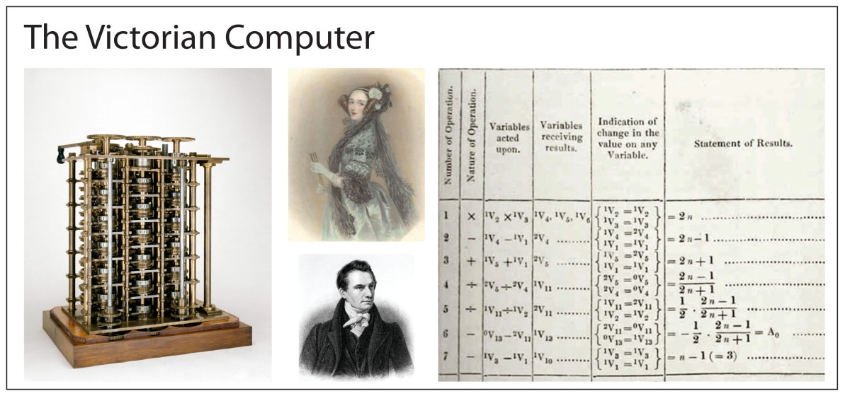
This working section of the Difference Engine can be seen today in the London Science Museum.  It is a marvel of steel and brass, consisting of three columns of stacked gears whose enmeshed teeth represent digital numbers.  As a crank handle is turned, the teath work upon each other, generating new numbers through the permutations of rotated gear teeth.  Carrying tens was initially a problem for Babbage, as it is for school children today, but he designed an ingenious mechanical system to accomplish the carry.

Fig. 3 One-seventh part of Babbage’s Difference Engine.

All was going well, and the government was pleased with progress, until Charles had a better idea that threatened to scrap all he had achieved.  It is not known how this new idea came into being, but it is known that it happened shortly after he met the amazing young woman: Ada Byron.

Lovely Lovelace

Ada Lovelace, born Ada Byron, had the awkward distinction of being the only legitimate child of Lord Byron, lyric genius and poet.  Such was Lord Byron’s hedonist lifestyle that no-one can say for sure how many siblings Ada had, not even Lord Byron himself, which was even more awkward when his half-sister bore a bastard child that may have been his.

Fig. 4 Ada Lovelace

Ada’s high-born mother prudently divorced the wayward poet and was not about to have Ada pulled into her father’s morass.  Where Lord Byron was bewitched (some would say possessed) by art and spirit, the mother sought an antidote, and she encouraged Ada to study hard cold mathematics.  She could not have known that Ada too had a genius like her father’s, only aimed differently, bewitched by the beauty in the sublime symbols of math. 

An insight into the precocious child’s way of thinking can be gained from a letter that the 12-year-old girl wrote to her mother who was off looking for miracle cures for imaginary ills. At that time in 1828, in a confluence of historical timelines in the history of mathematics, Ada and her mother (and Ada’s cat Puff) were living at Bifrons House which was the former estate of Brook Taylor, who had developed the Taylor’s series a hundred years earlier in 1715. In Ada’s letter, she describes a dream she had of a flying machine, which is not so remarkable, but then she outlined her plan to her mother to actually make one, which is remarkable. As you read her letter, you see she is already thinking about weights and material strengths and energy efficiencies, thinking like an engineer and designer—at the age of only 12 years!

In later years, Lovelace would become the Enchantress of Number to a number of her mathematical friends, one of whom was the strange man she met at a dinner party in the summer of 1833 when she was 17 years old.  The strange man was Charles Babbage, and when he talked to her about his Difference Engine, expecting to be tolerated as an entertaining side show, she asked pertinent questions, one after another, and the two became locked in conversation. 

Babbage was a recent widower, having lost his wife with whom he had been happily compatible, and one can only imagine how he felt when the attractive and intelligent woman gave him her attention.  But Ada’s mother would never see Charles as a suitable husband for her daughter—she had ambitious plans for her, and she tolerated Babbage only as much as she did because of the affection that Ada had for him.  Nonetheless, Ada and Charles became very close as friends and met frequently and wrote long letters to each other, discussing problems and progress on the Difference Engine.

In December of 1834, Charles invited Lady Byron and Ada to his home where he described with great enthusiasm a vision he had of an even greater machine.  He called it his Analytical Engine, and it would surpass his Difference Engine in a crucial way:  where the Difference Engine needed to be reconfigured by hand before every new calculation, the Analytical Engine would never need to be touched, it just needed to be programmed with punched cards.  Charles was in top form as he wove his narrative, and even Lady Byron was caught up in his enthusiasm.  The effect on Ada, however, was nothing less than a religious conversion. 

Fig. 5 General block diagram of Babbage’s Analytical Engine. From [8].

Ada’s Notes

To meet Babbage as an equal, Lovelace began to study mathematics with an obsession, or one might say, with delusions of grandeur.  She wrote “I believe myself to possess a most singular combination of qualities exactly fitted to make me pre-eminently a discoverer of the hidden realities of nature,” and she was convinced that she was destined to do great things.

Then, in 1835, Ada was married off to a rich but dull aristocrat who was elevated by royal decree to the Earldom of Lovelace, making her the Countess of Lovelace.  The marriage had little effect on Charles’ and Ada’s relationship, and he was invited frequently to the new home where they continued their discussions about the Analytical Engine. 

By this time Charles had informed the British government that he was putting all his effort into the design his new machine—news that was not received favorably since he had never delivered even a working Difference Engine.  Just when he hoped to start work on his Analytical Engine, the government ministers pulled their money. This began a decade’s long ordeal for Babbage as he continued to try to get monetary support as well as professional recognition from his peers for his ideas. Neither attempt was successful at home in Britain, but he did receive interest abroad, especially from a future prime minister of Italy, Luigi Menabrae, who invited Babbage to give a lecture in Turin on his Analytical Engine. Menabrae later had the lecture notes published in French. When Charles Wheatstone, a friend of Babbage, learned of Menabrae’s publication, he suggested to Lovelace that she translate it into English. Menabrae’s publication was the only existing exposition of the Analytical Engine, because Babbage had never written on the Engine himself, and Wheatstone was well aware of Lovelace’s talents, expecting her to be one of the only people in England who had the ability and the connections to Babbage to accomplish the task.

Ada Lovelace dove into the translation of Menabrae’s “Sketch of the Analytical Engine Invented by Charles Babbage” with the single-mindedness that she was known for. Along with the translation, she expanded on the work with Notes of her own that she added, lettered from A to G. By the time she wrote them, Lovelace had become a top-rate mathematician, possibly surpassing even Babbage, and her Notes were three times longer than the translation itself, providing specific technical details and mathematical examples that Babbage and Menabrae only allude to.

On a different level, the character of Ada’s Notes stands in stark contrast to Charles’ exposition as captured by Menabrae: where Menabrae provided only technical details of Babbage’s Engine, Lovelace’s Notes captured the Engine’s potential. She was still a poet by disposition—that inheritance from her father was never lost.

Lovelace wrote:

We may say most aptly, that the Analytical Engine weaves algebraic patterns just as the Jacquard-loom weaves flowers and leaves.

Here she is referring to the punched cards that the Jacquard loom used to program the weaving of intricate patterns into cloth. Babbage had explicitly borrowed this function from Jacquard, adapting it to provide the programmed input to his Analytical Engine.

But it was not all poetics. She also saw the abstract capabilities of the Engine, writing

In studying the action of the Analytical Engine, we find that the peculiar and independent nature of the considerations which in all mathematical analysis belong to operations, as distinguished from the objects operated upon and from the results of the operations performed upon those objects, is very strikingly defined and separated.

Again, it might act upon other things besides number, where objects found whose mutual fundamental relations could be expressed by those of the abstract science of operations, and which should be also susceptible of adaptations to the action of the operating notation and mechanism of the engine.

Supposing, for instance, that the fundamental relations of pitched sounds in the science of harmony and of musical composition were susceptible of such expression and adaptations, the engine might compose elaborate and scientific pieces of music of any degree of complexity or extent.

Here she anticipates computers generating musical scores.

Most striking is Note G. This is where she explicitly describes how the Engine would be used to compute numerical values as solutions to complicated problems. She chose, as her own example, the calculation of Bernoulli numbers which require extensive numerical calculations that were exceptionally challenging even for the best human computers of the day. In Note G, Lovelace writes down the step-by-step process by which the Engine would be programmed by the Jacquard cards to carry out the calculations. In the history of computer science, this stands as the first computer program.

Fig. 6 Table from Lovelace’s Note G on her method to calculate Bernoulli numbers using the Analytical Engine.

When it was time to publish, Babbage read over Lovelace’s notes, checking for accuracy, but he appears to have been uninterested in her speculations, possibly simply glossing over them. He saw his engine as a calculating machine for practical applications. She saw it for what we know today to be the exceptional adaptability of computers to all realms of human study and activity. He did not see what she saw. He was consumed by his Engine to the same degree as she, but where she yearned for the extraordinary, he sought funding for the mundane costs of machining and materials.

Ada’s Business Plan Pitch

Ada Lovelace watched in exasperation as Babbage floundered about with ill-considered proposals to the government while making no real progress towards a working Analytical Engine. Because of her vision into the potential of the Engine, a vision that struck her to her core, and seeing a prime opportunity to satisfy her own yearning to make an indelible mark on the world, she despaired in ever seeing it brought to fruition. Charles, despite his genius, was too impractical, wasting too much time on dead ends and incapable of performing the deft political dances needed to attract support. She, on the other hand, saw the project clearly and had the time and money and the talent, both mathematically and through her social skills, to help.

On Monday August 14, 1843, Ada wrote what might be the most heart-felt and impassioned business proposition in the history of computing. She laid out in clear terms to Charles how she could advance the Analytical Engine to completion if only he would surrender to her the day-to-day authority to make it happen. She was, in essence, proposing to be the Chief Operating Officer in a disruptive business endeavor that would revolutionize thinking machines a hundred years before their time. She wrote (she liked to underline a lot):

Firstly: I want to know whether if I continue to work on & about your own great subject, you will undertake to abide wholly by the judgment of myself (or of any persons whom you may now please to name as referees, whenever we may differ), on all practical matters relating to whatever can involve relations with any fellow-creature or fellow-creatures.

Secondly: can you undertake to give your mind wholly & undividedly, as a primary object that no engagement is to interfere with, to the consideration of all those matters in which I shall at times require your intellectual assistance & supervision; & can you promise not to slur & hurry things over; or to mislay, & allow confusion and mistakes to enter into documents, &c?

Thirdly: if I am able to lay before you in the course of a year or two, explicit & honorable propositions for executing your engine, (such as are approved by persons whom you may now name to be referred to for their approbation), would there be any chance of your allowing myself & such parties to conduct the business for you; your own undivided energies being devoted to the execution of the work; & all other matters being arranged for you on terms which your own friends should approve?

This is a remarkable letter from a self-possessed 28-year-old woman, laying out in explicit terms how she proposed to take on the direction of the project, shielding Babbage from the problems of relating to other people or “fellow-creatures” (which was his particular weakness), giving him time to focus his undivided attention on the technical details (which was his particular strength), while she would be the outward face of the project that would attract the appropriate funding.

In her preface to her letter, Ada adroitly acknowledges that she had been a romantic disappointment to Charles, but she pleads with him not to let their personal history cloud his response to her proposal. She also points out that her keen intellect would be an asset to the project and asks that he not dismiss it because of her sex (which a biased Victorian male would likely do). Despite her entreaties, this is exactly what Babbage did. Pencilled on the top of the original version of Ada’s letter in the Babbage archives is his simple note: “Tuesday 15 saw AAL this morning and refused all the conditions”. He had not even given her proposal 24 hours consideration as he indeed slurred and hurried things over.

Aftermath

Babbage never constructed his Analytical Engine and never even wrote anything about it. All his efforts would have been lost to history if Alan Turing had not picked up on Ada’s Notes and expanded upon them a hundred years later, bringing both her and him to the attention of the nascent computing community.

Ada Lovelace died young in 1852, at the age of 36, of cancer. By then she had moved on from Babbage and was working on other things. But she never was able to realize her ambition of uncovering such secrets of nature as to change the world.

Ada had felt from an early age that she was destined for greatness. She never achieved it in her lifetime and one can only wonder what she thought about this as she faced her death. Did she achieve it in posterity? This is a hotly debated question. Some say she wrote the first computer program, which may be true, but little programming a hundred years later derived directly from her work. She did not affect the trajectory of computing history. Discovering her work after the fact is interesting, but cannot be given causal weight in the history of science. The Vikings were the first Europeans to discover America, but no-one knew about it. They did not affect subsequent history the way that Columbus did.

On the other hand, Ada has achieved greatness in a different way. Now that her story is known, she stands as an exemplar of what scientific and technical opportunities look like, and the risk of ignoring them. Babbage also did not achieve greatness during his lifetime, but he could have—if he had not dismissed her and her intellect. He went to his grave embittered rather than lauded because he passed up an opportunity he never recognized.

By David D. Nolte, June 26, 2023


References

[1] Facsimile of “Sketch of the Analytical Engine Invented by Charles Babbage” translated by Ada Lovelace from Harvard University.

[2] Facsimile of Ada Lovelace’s “Notes by the Translator“.

[3] Stephen Wolfram, “Untangling the Tale of Ada Lovelace“, Wolfram Writings (2015).

[4] J. Essinger, “Charles and Ada : The computer’s most passionate partnership,” (History Press, 2019).

[5] D. Swade, The Difference Engine: Charles Babbage and the quest to build the first computer (Penguin Books, 2002).

[6] W. Gibson, and B. Sterling, The Difference Engine (Bantam Books, 1992).

[7] L. J. Snyder, The Philosophical Breakfast Club : Four remarkable friends who transformed science and changed the world (Broadway Books, 2011).

[8] Allan G. Bromley, Charles Babbage’s Analytical Engine, 1838, Annals of the History of Computing, Volume 4, Number 3, July 1982, pp. 196 – 217

Io, Europa, Ganymede, and Callisto: Galileo’s Moons in the History of Science

When Galileo trained his crude telescope on the planet Jupiter, hanging above the horizon in 1610, and observed moons orbiting a planet other than Earth, it created a quake whose waves have rippled down through the centuries to today.  Never had such hard evidence been found that supported the Copernican idea of non-Earth-centric orbits, freeing astronomy and cosmology from a thousand years of error that shaded how people thought.

The Earth, after all, was not the center of the Universe.

Galileo’s moons: the Galilean Moons—Io, Europa, Ganymede, and Callisto—have drawn our eyes skyward now for over 400 years.  They have been the crucible for numerous scientific discoveries, serving as a test bed for new ideas and new techniques, from the problem of longitude to the speed of light, from the birth of astronomical interferometry to the beginnings of exobiology.  Here is a short history of Galileo’s Moons in the history of physics.

Galileo (1610): Celestial Orbits

In late 1609, Galileo (1564 – 1642) received an unwelcome guest to his home in Padua—his mother.  She was not happy with his mistress, and she was not happy with his chosen profession, but she was happy to tell him so.  By the time she left in early January 1610, he was yearning for something to take his mind off his aggravations, and he happened to point his new 20x telescope in the direction of the planet Jupiter hanging above the horizon [1].  Jupiter appeared as a bright circular spot, but nearby were three little stars all in line with the planet.  The alignment caught his attention, and when he looked again the next night, the position of the stars had shifted.  On successive nights he saw them shift again, sometimes disappearing into Jupiter’s bright disk.  Several days later he realized that there was a fourth little star that was also behaving the same way.  At first confused, he had a flash of insight—the little stars were orbiting the planet.  He quickly understood that just as the Moon orbited the Earth, these new “Medicean Planets” were orbiting Jupiter.  In March 1610, Galileo published his findings in Siderius Nuncius (The Starry Messenger). 

Page from Galileo’s Starry Messenger showing the positions of the moon of Jupiter

It is rare in the history of science for there not to be a dispute over priority of discovery.  Therefore, by an odd chance of fate, on the same nights that Galileo was observing the moons of Jupiter with his telescope from Padua, the German astronomer Simon Marius (1573 – 1625) also was observing them through a telescope of his own from Bavaria.  It took Marius four years to publish his observations, long after Galileo’s Siderius had become a “best seller”, but Marius took the opportunity to claim priority.  When Galileo first learned of this, he called Marius “a poisonous reptile” and “an enemy of all mankind.”  But harsh words don’t settle disputes, and the conflicting claims of both astronomers stood until the early 1900’s when a scientific enquiry looked at the hard evidence.  By that same odd chance of fate that had compelled both men to look in the same direction around the same time, the first notes by Marius in his notebooks were dated to a single day after the first notes by Galileo!  Galileo’s priority survived, but Marius may have had the last laugh.  The eternal names of the “Galilean” moons—Io, Europe, Ganymede and Callisto—were given to them by Marius.

Picard and Cassini (1671):  Longitude

The 1600’s were the Age of Commerce for the European nations who relied almost exclusively on ships and navigation.  While latitude (North-South) was easily determined by measuring the highest angle of the sun above the southern horizon, longitude (East-West) relied on clocks which were notoriously inaccurate, especially at sea. 

The Problem of Determining Longitude at Sea is the subject of Dava Sobel’s thrilling book Longitude (Walker, 1995) [2] where she reintroduced the world to what was once the greatest scientific problem of the day.  Because almost all commerce was by ships, the determination of longitude at sea was sometimes the difference between arriving safely in port with a cargo or being shipwrecked.  Galileo knew this, and later in his life he made a proposal to the King of Spain to fund a scheme to use the timings of the eclipses of his moons around Jupiter to serve as a “celestial clock” for ships at sea.  Galileo’s grant proposal went unfunded, but the possibility of using the timings of Jupiter’s moons for geodesy remained an open possibility, one which the King of France took advantage of fifty years later.

In 1671 the newly founded Academie des Sciences in Paris funded an expedition to the site of Tycho Brahe’s Uranibourg Observatory in Hven, Denmark, to measure the time of the eclipses of the Galilean moons observed there to be compared the time of the eclipses observed in Paris by Giovanni Cassini (1625 – 1712).  When the leader of the expedition, Jean Picard (1620 – 1682), arrived in Denmark, he engaged the services of a local astronomer, Ole Rømer (1644 – 1710) to help with the observations of over 100 eclipses of the Galilean moon Io by the planet Jupiter.  After the expedition returned to France, Cassini and Rømer calculated the time differences between the observations in Paris and Hven and concluded that Galileo had been correct.  Unfortunately, observing eclipses of the tiny moon from the deck of a ship turned out not to be practical, so this was not the long-sought solution to the problem of longitude, but it contributed to the early science of astrometry (the metrical cousin of astronomy).  It also had an unexpected side effect that forever changed the science of light.

Ole Rømer (1676): The Speed of Light

Although the differences calculated by Cassini and Rømer between the times of the eclipses of the moon Io between Paris and Hven were small, on top of these differences was superposed a surprisingly large effect that was shared by both observations.  This was a systematic shift in the time of eclipse that grew to a maximum value of 22 minutes half a year after the closest approach of the Earth to Jupiter and then decreased back to the original time after a full year had passed and the Earth and Jupiter were again at their closest approach.  At first Cassini thought the effect might be caused by a finite speed to light, but he backed away from this conclusion because Galileo had shown that the speed of light was unmeasurably fast, and Cassini did not want to gainsay the old master.

Ole Rømer

Rømer, on the other hand, was less in awe of Galileo’s shadow, and he persisted in his calculations and concluded that the 22 minute shift was caused by the longer distance light had to travel when the Earth was farthest away from Jupiter relative to when it was closest.  He presented his results before the Academie in December 1676 where he announced that the speed of light, though very large, was in fact finite.  Unfortnately, Rømer did not have the dimensions of the solar system at his disposal to calculate an actual value for the speed of light, but the Dutch mathematician Huygens did.

When Huygens read the proceedings of the Academie in which Rømer had presented his findings, he took what he knew of the radius of Earth’s orbit and the distance to Jupiter and made the first calculation of the speed of light.  He found a value of 220,000 km/second (kilometers did not exist yet, but this is the equivalent of what he calculated).  This value is 26 percent smaller than the true value, but it was the first time a number was given to the finite speed of light—based fundamentally on the Galilean moons. For a popular account of the story of Picard and Rømer and Huygens and the speed of light, see Ref. [3].

Michelson (1891): Astronomical Interferometry

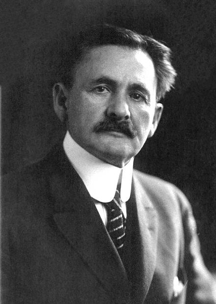
Albert Michelson (1852 – 1931) was the first American to win the Nobel Prize in Physics.  He received the award in 1907 for his work to replace the standard meter, based on a bar of metal housed in Paris, with the much more fundamental wavelength of red light emitted by Cadmium atoms.  His work in Paris came on the heels of a new and surprising demonstration of the use of interferometry to measure the size of astronomical objects.

Albert Michelson

The wavelength of light (a millionth of a meter) seems ill-matched to measuring the size of astronomical objects (thousands of meters) that are so far from Earth (billions of meters).  But this is where optical interferometry becomes so important.  Michelson realized that light from a distant object, like a Galilean moon of Jupiter, would retain some partial coherence that could be measured using optical interferometry.  Furthermore, by measuring how the interference depended on the separation of slits placed on the front of a telescope, it would be possible to determine the size of the astronomical object.

From left to right: Walter Adams, Albert Michelson, Walther Mayer, Albert Einstein, Max Ferrand, and Robert Milliken. Photo taken at Caltech.

In 1891, Michelson traveled to California where the Lick Observatory was poised high above the fog and dust of agricultural San Jose (a hundred years before San Jose became the capitol of high-tech Silicon Valley).  Working with the observatory staff, he was able to make several key observations of the Galilean moons of Jupiter.  These were just close enough that their sizes could be estimated (just barely) from conventional telescopes.  Michelson found from his calculations of the interference effects that the sizes of the moons matched the conventional sizes to within reasonable error.  This was the first demonstration of astronomical interferometry which has burgeoned into a huge sub-discipline of astronomy today—based originally on the Galilean moons [4].

Pioneer (1973 – 1974): The First Tour

Pioneer 10 was launched on March 3, 1972 and made its closest approach to Jupiter on Dec. 3, 1973. Pioneer 11 was launched on April 5, 1973 and made its closest approach to Jupiter on Dec. 3, 1974 and later was the first spacecraft to fly by Saturn. The Pioneer spacecrafts were the first to leave the solar system (there have now been 5 that have left, or will leave, the solar system). The cameras on the Pioneers were single-pixel instruments that made line-scans as the spacecraft rotated. The point light detector was a Bendix Channeltron photomultiplier detector, which was a vacuum tube device (yes vacuum tube!) operating at a single-photon detection efficiency of around 10%. At the time of the system design, this was a state-of-the-art photon detector. The line scanning was sufficient to produce dramatic photographs (after extensive processing) of the giant planets. The much smaller moons were seen with low resolution, but were still the first close-ups ever to be made of Galileo’s moons.

Voyager (1979): The Grand Tour

Voyager 1 was launched on Sept. 5, 1977 and Voyager 2 was launched on August 20, 1977. Although Voyager 1 was launched second, it was the first to reach Jupiter with closest approach on March 5, 1979. Voyager 2 made its closest approach to Jupiter on July 9, 1979.

In the Fall of 1979, I had the good fortune to be an undergraduate at Cornell University when Carl Sagan gave an evening public lecture on the Voyager fly-bys, revealing for the first time the amazing photographs of not only Jupiter but of the Galilean Moons. Sitting in the audience listening to Sagan, a grand master of scientific story telling, made you feel like you were a part of history. I have never been so convinced of the beauty and power of science and technology as I was sitting in the audience that evening.

The camera technology on the Voyagers was a giant leap forward compared to the Pioneer spacecraft. The Voyagers used cathode ray vidicon cameras, like those used in television cameras of the day, with high-resolution imaging capabilities. The images were spectacular, displaying alien worlds in high-def for the first time in human history: volcanos and lava flows on the moon of Io; planet-long cracks in the ice-covered surface of Europa; Callisto’s pock-marked surface; Ganymede’s eerie colors.

The Voyager’s discoveries concerning the Galilean Moons were literally out of this world. Io was discovered to be a molten planet, its interior liquified by tidal-force heating from its nearness to Jupiter, spewing out sulfur lava onto a yellowed terrain pockmarked by hundreds of volcanoes, sporting mountains higher than Mt. Everest. Europa, by contrast, was discovered to have a vast flat surface of frozen ice, containing no craters nor mountains, yet fractured by planet-scale ruptures stained tan (for unknown reasons) against the white ice. Ganymede, the largest moon in the solar system, is a small planet, larger than Mercury. The Voyagers revealed that it had a blotchy surface with dark cratered patches interspersed with light smoother patches. Callisto, again by contrast, was found to be the most heavily cratered moon in the solar system, with its surface pocked by countless craters.

Galileo (1995): First in Orbit

The first mission to orbit Jupiter was the Galileo spacecraft that was launched, not from the Earth, but from Earth orbit after being delivered there by the Space Shuttle Atlantis on Oct. 18, 1989. Galileo arrived at Jupiter on Dec. 7, 1995 and was inserted into a highly elliptical orbit that became successively less eccentric on each pass. It orbited Jupiter for 8 years before it was purposely crashed into the planet (to prevent it from accidentally contaminating Europa that may support some form of life).

Galileo made many close passes to the Galilean Moons, providing exquisite images of the moon surfaces while its other instruments made scientific measurements of mass and composition. This was the first true extended study of Galileo’s Moons, establishing the likely internal structures, including the liquid water ocean lying below the frozen surface of Europa. As the largest body of liquid water outside the Earth, it has been suggested that some form of life could have evolved there (or possibly been seeded by meteor ejecta from Earth).

Juno (2016): Still Flying

The Juno spacecraft was launched from Cape Canaveral on Aug. 5, 2011 and entered a Jupiter polar orbit on July 5, 2016. The mission has been producing high-resolution studies of the planet. The mission was extended in 2021 to last to 2025 to include several close fly-bys of the Galilean Moons, especially Europa, which will be the object of several upcoming missions because of the possibility for the planet to support evolved life. These future missions include NASA’s Europa Clipper Mission, the ESA’s Jupiter Icy Moons Explorer, and the Io Volcano Observer.

Epilog (2060): Colonization of Callisto

In 2003, NASA identified the moon Callisto as the proposed site of a manned base for the exploration of the outer solar system. It would be the next most distant human base to be established after Mars, with a possible start date by the mid-point of this century. Callisto was chosen because it is has a low radiation level (being the farthest from Jupiter of the large moons) and is geologically stable. It also has a composition that could be mined to manufacture rocket fuel. The base would be a short-term way-station (crews would stay for no longer than a month) for refueling before launching and using a gravity assist from Jupiter to sling-shot spaceships to the outer planets.

By David D. Nolte, May 29, 2023


[1] See Chapter 2, A New Scientist: Introducing Galileo, in David D. Nolte, Galileo Unbound (Oxford University Press, 2018).

[2] Dava Sobel, Longitude: The True Story of a Lone Genius who Solved the Greatest Scientific Problem of his Time (Walker, 1995)

[3] See Chap. 1, Thomas Young Polymath: The Law of Interference, in David D. Nolte, Interference: The History of Optical Interferometry and the Scientists who Tamed Light (Oxford University Press, 2023)

[4] See Chapter 5, Stellar Interference: Measuring the Stars, in David D. Nolte, Interference: The History of Optical Interferometry and the Scientists who Tamed Light (Oxford University Press, 2023).

The Mighty Simplex

There is no greater geometric solid than the simplex.  It is the paragon of efficiency, the pinnacle of symmetry, and the prototype of simplicity.  If the universe were not constructed of continuous coordinates, then surely it would be tiled by tessellations of simplices.

Indeed, simplices, or simplexes, arise in a wide range of geometrical problems and real-world applications.  For instance, metallic alloys are described on a simplex to identify the constituent elements [1].  Zero-sum games in game theory and ecosystems in population dynamics are described on simplexes [2], and the Dantzig simplex algorithm is a central algorithm for optimization in linear programming [3].  Simplexes also are used in nonlinear minimization (amoeba algorithm), in classification problems in machine learning, and they also raise their heads in quantum gravity.  These applications reflect the special status of the simplex in the geometry of high dimensions.

… It’s Simplexes all the way down!

The reason for their usefulness is the simplicity of their construction that guarantees a primitive set that is always convex.  For instance, in any space of d-dimensions, the simplest geometric figure that can be constructed of flat faces to enclose a d-volume consists of d+1 points that is the d-simplex. 

Or …

In any space of d-dimensions, the simplex is the geometric figure whose faces are simplexes, whose faces are simplexes, whose faces are again simplexes, and those faces are once more simplexes … And so on. 

In other words, it’s simplexes all the way down.

Simplex Geometry

In this blog, I will restrict the geometry to the regular simplex.  The regular simplex is the queen of simplexes: it is the equilateral simplex for which all vertices are equivalent, and all faces are congruent, and all sub-faces are congruent, and so on.  The regular simplexes have the highest symmetry properties of any polytope. A polytope is the d-dimensional generalization of a polyhedron.  For instance, the regular 2-simplex is the equilateral triangle, and the regular 3-simplex is the equilateral tetrahedron.

The N-simplex is the high-dimensional generalization of the tetrahedron.  It is a regular N-dimensional polytope with N+1 vertexes.  Starting at the bottom and going up, the simplexes are the point (0-simplex), the unit line (1-simplex), the equilateral triangle (2-simplex), the tetrahedron (3-simplex), the pentachoron (4-simplex), the hexateron (5-simplex) and onward.  When drawn on the two-dimensional plane, the simplexes are complete graphs with links connecting every node to every other node.  This dual character of equidistance and completeness give simplexes their utility. Each node is equivalent and is linked to each other.  There are N•(N-1)/2 links among N vertices, and there are (N-2)•(N-1)/2 triangular faces.

Fig. 1  The N-simplex structures from 1-D through 10-D.  Drawn on the 2D plane, the simplexes are complete graphs with links between every node.  The number of vertices is equal to the number of dimensions plus one. (Wikipedia)
Fig. 2 Coulomb-spring visualization of the energy minimization of a 12-simplex (a 12-dimensional tetrahedron). Each node is a charge. Each link is a spring. Beginning as a complete graph on the planar circle, it finds a minimum configuration with 3 internal nodes.

Construction of a d-simplex is recursive:  Begin with a (d-1)-dimensional simplex and add a point along an orthogonal dimension to construct a d-simplex.  For instance, to create a 2-simplex (an equilateral triangle), find the mid-point of the 1-simplex (a line segment)

            Centered 1-simplex:                (-1), (1)    

add a point on the perpendicular that is the same distance from each original vertex as the original vertices were distant from each other     

            Off-centered 2-simplex:         (-1,0), (1,0), (0, sqrt(3)/2)

Then shift the origin to the center of mass of the triangle

            Centered 2-simplex:               (-1, -sqrt(3)/6), (1, -sqrt(3)/6), (0, sqrt(3)/3)

The 2-simplex, i.e., the equilateral triangle, has a 1-simplex as each of its faces.  And each of those 1-simplexes has a 0-simplex as each of its ends.  Therefore, this recursive construction of ever higher-dimensional simplexes out of low-dimensional ones, provides an interesting pattern:

Fig. 3 The entries are the same numbers that appear in Pascal’s Triangle. (Wikipedia)

The coordinates of an N-simplex are not unique, although there are several convenient conventions.  One convention defines standard coordinates for an N-simplex in N+1 coordinate bases.  These coordinates embed the simplex into a space of one higher dimension.  For instance, the standard 2-simplex is defined by the coordinates (001), (010), (100) forming a two-dimensional triangle in three dimensions, and the simplex is a submanifold in the embedding space.  A more efficient coordinate choice matches the coordinate-space dimensionality to the dimensionality of the simplex.  Hence the 10 vertices of a 9-simplex can be defined by 9 coordinates (also not unique).  One choice is given in Fig. 4 for the 1-simplex up to the 9-simplex. 

Fig. 4 One possible set of coordinates for the 1-simplex up to the 9-simplex.  The center of mass of the simplex is at the origin, and the edge lengths are equal to 2.

The equations for the simplex coordinates are

where

is the “diagonal” vector.  These coordinates are centered on the center of mass of the simplex, and the links all have length equal to 2 which can be rescaled by a multiplying factor.  The internal dihedral angle between all of the coordinate vectors for an N-simplex is

For moderate to high-dimensionality, the position vectors of the simplex vertices are pseudo-orthogonal.  For instance, for N = 9 the dihedral angle cosine is -1/9 = -0.111.  For higher dimensions, the simplex position vectors become asymptotically orthogonal.  Such orthogonality is an important feature for orthonormal decomposition of class superpositions, for instance of overlapping images.

Alloy Mixtures and Barycentric Coordinates

For linear systems, the orthonormality of basis representations is one of the most powerful features for system analysis in terms of superposition of normal modes.  Neural networks, on the other hand, are intrinsically nonlinear decision systems for which linear superposition does not hold inside the network, even if the symbols presented to the network are orthonormal superpositions.  This loss of orthonormality in deep networks can be partially retrieved by selecting the Simplex code.  It has pseudo-orthogonal probability distribution functions located on the vertices of the simplex.  There is an additional advantage to using the Simplex code: by using so-called barycentric coordinates, the simplex vertices can be expressed as independent bases.  An example for the 2-simplex is shown in Fig. 5.  The x-y Cartesian coordinates of the vertices (using tensor index notation) are given by (S11, S12), (S21, S22), and (S31, S32).  Any point (x1, x2) on the plane can be expressed as a linear combination of the three vertices with barycentric coordinates (v1, v2, v3) by solving for these three coefficients from the equation

using Cramers rule.  For instance, the three vertices of the simplex are expressed using the 3-component barycentric coordinates (1,0,0), (0,1,0) and (0,0,1).  The mid-points on the edges have barycentric coordinates (1/2,1/2,0), (0,1/2,1/2), and (1/2,0,1/2).  The centroid of the simplex has barycentric coordinates (1/3,1/3,1/3).  Barycentric coordinates on a simplex are commonly used in phase diagrams of alloy systems in materials science. The simplex can also be used to identify crystallographic directions in three-dimensions, as in Fig. 6.

Fig. 5  Barycentric coordinates on the 2-Simplex.  The vertices represent “orthogonal” pure symbols.  Superpositions of 2 symbols lie on the edges.  Any point on the simplex can be represented using barycentric coordinates with three indices corresponding to the mixture of the three symbols.
Fig. 6 Crystallographic orientations expressed on a simplex. From A Treatise on Crystallography, William Miller, Cambridge (1839)

Replicator Dynamics on the Simplex

Ecosystems are among the most complex systems on Earth.  The complex interactions among hundreds or thousands of species may lead to steady homeostasis in some cases, to growth and collapse in other cases, and to oscillations or chaos in yet others.  But the definition of species can be broad and abstract, referring to businesses and markets in economic ecosystems, or to cliches and acquaintances in social ecosystems, among many other examples.  These systems are governed by the laws of evolutionary dynamics that include fitness and survival as well as adaptation. The dimensionality of the dynamical spaces for these systems extends to hundreds or thousands of dimensions—far too complex to visualize when thinking in four dimensions is already challenging. 

A classic model of interacting species is the replicator equation. It allows for a fitness-based proliferation and for trade-offs among the individual species. The replicator dynamics equations are shown in Fig. 7.

Fig. 7 Replicator dynamics has a surprisingly simple form, but with surprisingly complicated behavior. The key elements are the fitness and the payoff matrix. The fitness relates to how likely the species will survive. The payoff matrix describes how one species gains at the loss of another (although symbiotic relationships also occur).

The population dynamics on the 2D simplex are shown in Fig. 8 for several different pay-off matrices (square matrix to the upper left of each simplex). The matrix values are shown in color and help interpret the trajectories. For instance the simplex on the upper-right shows a fixed point center. This reflects the antisymmetric character of the pay-off matrix around the diagonal. The stable spiral on the lower-left has a nearly asymmetric pay-off matrix, but with unequal off-diagonal magnitudes. The other two cases show central saddle points with stable fixed points on the boundary. A large variety of behaviors are possible for this very simple system. The Python program can be found in Trirep.py.

Fig. 8 Payoff matrix and population simplex for four random cases: Upper left is an unstable saddle. Upper right is a center. Lower left is a stable spiral. Lower right is a marginal case.

Linear Programming with the Dantzig Simplex

There is a large set of optimization problems in which a linear objective function is to be minimized subject to a set of inequalities. This is known as “Linear Programming”. These LP systems can be expressed as

The vector index goes from 1 to d, the dimension of the space. Each inequality creates a hyperplane, where two such hyperplanes intersect along a line terminated at each end by a vertex point. The set of vertexes defines a polytope in d-dimensions, and each face of the polytope, when combined with the point at the origin, defines a 3-simplex.

It is easy to visualize in lower dimensions why the linear objective function must have an absolute minimum at one of the vertexes of the polytope. And finding that minimum is a trivial exercise: Start at any vertex. Poll each neighboring vertex and move to the one that has the lowest value of the objective function. Repeat until the current vertex has a lower objective value than any neighbors. Because of the linearity of the objective function, this is a unique minimum (except for rare cases of accidental degeneracy). This iterative algorithm defines a walk on the vertexes of the polytope.

The question arises, why not just evaluate the objection function at each vertex and then just pick the vertex with the lowest value? The answer in high dimensions is that there are too many vertexes, and finding all of them is inefficient. If there are N vertexes, the walk to the solution visits only a few of the vertexes, on the order of log(N). The algorithm therefore scales as log(N), just like a search tree.

Fig. 9 Dantzig simplex approach on a convex 3D space of basic solutions in a linear programming problem.

This simple algorithm was devised by George Dantzig (1914 – 2005) in 1939 when he was a graduate student at UC Berkeley. He had arrived late to class and saw two problems written on the chalk board. He assumed that these were homework assignments, so he wrote them down and worked on them over the following week. He recalled that they seemed a bit harder than usual, but he eventually solved them and turned them in. A few weeks later, his very excited professor approached him and told him that the problems weren’t homework–they were two of the most important outstanding problems in optimization and that Dantzig had just solved them! The 1997 movie Good Will Hunting, with Matt Damon, Ben Affleck, and Robin Williams, borrowed this story for the opening scene.

The Amoeba Simplex Crawling through Hyperspace

Unlike linear programming problems with linear objective functions, multidimensional minimization of nonlinear objective functions is an art unto itself, with many approach. One of these is a visually compelling algorithm that does the trick more often than not. This is the so-called amoeba algorithm that shares much in common with the Dantzig simplex approach to linear programming, but instead of a set of fixed simplex coordinates, it uses a constantly shifting d-dimensional simplex that “crawls” over the objective function, seeking its minimum.

One of the best descriptions of the amoeba simplex algorithm is in “Numerical Recipes” [4] that describes the crawling simplex as

When it reaches a “valley floor”, the method contracts itself in the transverse direction and tries to ooze down the valley. If there is a situation where the simplex is trying to “pass through the eye of a needle”, it contracts itself in all directions, pulling itself in around its lowest (best) point.

(From Press, Numerical Recipes, Cambridge)

The basic operations for the crawling simplex are reflection and scaling. For a given evaluation of all the vertexes of the simplex, one will have the highest value and another the lowest. In a reflection, the highest point is reflected through the d-dimensional face defined by the other d vertexes. After reflection, if the new evaluation is lower than the former lowest value, then the point is expanded. If, on the other hand, it is little better than it was before reflection, then the point is contracted. The expansion and contraction are what allows the algorithm to slide through valleys or shrink to pass through the eye of a needle.

The amoeba algorithm was developed by John Nelder and Roger Mead in 1965 at a time when computing power was very limited. The algorithm works great as a first pass at a minimization problem, and it almost always works for moderately small dimensions, but for very high dimensions there are more powerful algorithms today for optimization, built into all the deep learning software environments like Tensor Flow and the Matlab toolbox.

By David D. Nolte, May 3, 2023


[1] M. Hillert, Phase equilibria, phase diagrams and phase transformations : their thermodynamic basis.  (Cambridge University Press, Cambridge, UK ;, ed. 2nd ed., 2008).

[2] P. Schuster, K. Sigmund, Replicator Dynamics. Journal of Theoretical Biology 100, 533-538 (1983); P. Godfrey-Smith, The replicator in retrospect. Biology & Philosophy 15, 403-423 (2000).

[3] R. E. Stone, C. A. Tovey, The Simplex and Projective Scaling Algorithms as Iteratively Reweighted Least-squares Methods. Siam Review 33, 220-237 (1991).

[4] W. H. Press, Numerical Recipes in C++ : The Art of Scientific Computing.  (Cambridge University Press, Cambridge, UK; 2nd ed., 2002).

From Coal and Steam to ChatGPT: Chapters in the History of Technology

Mark Twain once famously wrote in a letter from London to a New York newspaper editor:

“I have … heard on good authority that I was dead [but] the report of my death was an exaggeration.”

The same may be true of recent reports on the grave illness and possible impending death of human culture at the hands of ChatGPT and other so-called Large Language Models (LLM).  It is argued that these algorithms have such sophisticated access to the bulk of human knowledge, and can write with apparent authority on virtually any topic, that no-one needs to learn or create anything new. It can all be recycled—the end of human culture!

While there may be a kernel of truth to these reports, they are premature.  ChatGPT is just the latest in a continuing string of advances that have disrupted human life and human culture ever since the invention of the steam engine.  We—humans, that is—weathered the steam engine in the short term and are just as likely to weather the LLM’s. 

ChatGPT: What is it?

For all the hype, ChatGPT is mainly just a very sophisticated statistical language model (SLM). 

To start with a very simple example of SLM, imagine you are playing a word scramble game and have the letter “Q”. You can be pretty certain that the “Q“ will be followed by a “U” to make “QU”.  Or if you have the initial pair “TH” there is a very high probability that it will be followed by a vowel as “THA…”, “THE…”, ”THI…”, “THO..” or “THU…” and possibly with an “R” as “THR…”.  This almost exhausts the probabilities.  This is all determined by the statistical properties of English.

Statistical language models build probability distributions for the likelihood that some sequence of letters will be followed by another sequence of letters, or a sequence of words (and punctuations) will be followed by another sequence of words.  The bigger the chains of letters and words, the number of possible permutations grows exponentially.  This is why SLMs usually stop at some moderate order of statistics.  If you build sentences from such a model, it sounds OK for a sentence or two, but then it just drifts around like it’s dreaming or hallucinating in a stream of consciousness without any coherence.

ChatGPT works in much the same way.  It just extends the length of the sequences where it sounds coherent up to a paragraph or two.  In this sense, it is no more “intelligent” than the SLM that follows “Q” with “U”.  ChatGPT simply sustains the charade longer.

Now the details of how ChatGPT accomplishes this charade is nothing less than revolutionary.  The acronym GPT means Generative Pre-Trained Transformer.  Transformers were a new type of neural net architecture invented in 2017 by the Google Brain team.  Transformers removed the need to feed sentences word-by-word into a neural net, instead allowing whole sentences and even whole paragraphs to be input in parallel.  Then, by feeding the transformers on more than a Terabyte of textual data from the web, they absorbed the vast output of virtually all the crowd-sourced information from the past 20 years.  (This what transformed the model from an SLM to an LLM.)  Finally, using humans to provide scores on what good answers looked like versus bad answers, ChatGPT was supervised to provide human-like responses.  The result is a chatbot that in any practical sense passes the Turing Test—if you query it for an extended period of time, you would be hard pressed to decide if it was a computer program or a human giving you the answers.  But Turing Tests are boring and not very useful. 

Figure. The Transformer architecture broken into the training step and the generation step. In training, pairs of inputs and targets are used to train encoders and decoders to build up word probabilities at the output. In generation, a partial input, or a query, is presented to the decoders that find the most likely missing, or next, word in the sequence. The sentence is built up sequentially in each iteration. It is an important distinction that this is not a look-up table … it is trained on huge amounts of data and learns statistical likelihoods, not exact sequences.

The true value of ChatGPT is the access it has to that vast wealth of information (note it is information and not knowledge).  Give it almost any moderately technical query, and it will provide a coherent summary for you—on amazingly esoteric topics—because almost every esoteric topic has found its way onto the net by now, and ChatGPT can find it. 

As a form of search engine, this is tremendous!  Think how frustrating it has always been searching the web for something specific.  Furthermore, the lengthened coherence made possible by the transformer neural net means that a first query that leads to an unsatisfactory answer from the chatbot can be refined, and ChatGPT will find a “better” response, conditioned by the statistics of its first response that was not optimal.  In a feedback cycle, with the user in the loop, very specific information can be isolated.

Or, imagine that you are not a strong writer, or don’t know the English language as well as you would like.  But entering your own text, you can ask ChatGPT to do a copy-edit, even rephrasing your writing where necessary, because ChatGPT above all else has an unequaled command of the structure of English.

Or, for customer service, instead of the frustratingly discrete menu of 5 or 10 potted topics, ChatGPT with a voice synthesizer could respond to continuously finely graded nuances of the customer’s problem—not with any understanding or intelligence, but with probabilistic likelihoods of what the solutions are for a broad range of possible customer problems.

In the midst of all the hype surrounding ChatGPT, it is important to keep in mind two things:  First, we are witnessing the beginning of a revolution and a disruptive technology that will change how we live.  Second, it is still very early days, just like the early days of the first steam engines running on coal.

Disruptive Technology

Disruptive technologies are the coin of the high-tech realm of Silicon Valley.  But this is nothing new.  There have always been disruptive technologies—all the way back to Thomas Newcomen and James Watt and the steam engines they developed between 1712 and 1776 in England.  At first, steam engines were so crude they were used only to drain water from mines, increasing the number jobs in and around the copper and tin mines of Cornwall (viz. the popular BBC series Poldark) and the coal mines of northern England.  But over the next 50 years, steam engines improved, and they became the power source for textile factories that displaced the cottage industry of spinning and weaving that had sustained marginal farms for centuries before.

There is a pattern to a disruptive technology.  It not only disrupts an existing economic model, but it displaces human workers.  Once-plentiful jobs in an economic sector can vanish quickly after the introduction of the new technology.  The change can happen so fast, that there is not enough time for the workforce to adapt, followed by human misery in some sectors.  Yet other, newer, sectors always flourish, with new jobs, new opportunities, and new wealth.  The displaced workers often never see these benefits because they lack skills for the new jobs. 

The same is likely true for the LLMs and the new market models they will launch. There will be a wealth of new jobs curating and editing LLM outputs. There will also be new jobs in the generation of annotated data and in the technical fields surrounding the support of LLMs. LLMs are incredibly hungry for high-quality annotated data in a form best provided by humans. Jobs unlikely to be at risk, despite prophesies of doom, include teachers who can use ChatGPT as an aide by providing appropriate context to its answers. Conversely, jobs that require a human to assemble information will likely disappear, such as news aggregators. The same will be true of jobs in which effort is repeated, or which follow a set of patterns, such as some computer coding jobs or data analysts. Customer service positions will continue to erode, as will library services. Media jobs are at risk, as well as technical writing. The writing of legal briefs may be taken over by LLMs, along with market and financial analysts. By some estimates, there are 300 million jobs around the world that will be impacted one way or another by the coming spectrum of LLMs.

This pattern of disruption is so set and so clear and so consistent, that forward-looking politicians or city and state planners could plan ahead, because we have been on a path of continuing waves disruption for over two hundred years.

Waves of Disruption

In the history of technology, it is common to describe a series of revolutions as if they were distinct.  The list looks something like this:

First:          Power (The Industrial Revolution: 1760 – 1840)

Second:     Electricity and Connectivity (Technological Revolution: 1860 – 1920)

Third:        Automation, Information, Cybernetics (Digital Revolution: 1950 – )

Fourth:      Intelligence, cyber-physical (Imagination Revolution: 2010 – )

The first revolution revolved around steam power fueled by coal, radically increasing output of goods.  The second revolution shifted to electrical technologies, including communication networks through telegraph and the telephones.  The third revolution focused on automation and digital information.

Yet this discrete list belies an underlying fact:  There is, and has been, only one continuous Industrial Revolution punctuated by waves.

The Age of Industrial Revolutions began around 1760 with the invention of the spinning jenny by James Hargreaves—and that Age has continued, almost without pause, up to today and will go beyond.  Each disruptive technology has displaced the last.  Each newly trained workforce has been displaced by the last.  The waves keep coming. 

Note that the fourth wave is happening now, as artificial intelligence matures. This is ironic, because this latest wave of the Industrial Revolution is referred to as the “Imagination Revolution” by the optimists who believe that we are moving into a period where human creativity is unleashed by the unlimited resources of human connectivity across the web. Yet this moment of human ascension to the heights of creativity is happening at just the moment when LLM’s are threatening to remove the need to create anything new.

So is it the end of human culture? Will all knowledge now just be recycled with nothing new added?

A Post-Human Future?

The limitations of the generative aspects of ChatGPT might be best visualized by using an image-based generative algorithm that has also gotten a lot of attention lately. This is the ability to input a photograph, and input a Van Gogh painting, and create a new painting of the photograph in the style of Van Gogh.

In this example, the output on the right looks like a Van Gogh painting. It is even recognizable as a Van Gogh. But in fact it is a parody. Van Gogh consciously created something never before seen by humans.

Even if an algorithm can create “new” art, it is a type of “found” art, like a picturesque stone formation or a sunset. The beauty becomes real only in the response it elicits in the human viewer. Art and beauty do not exist by themselves; they only exist in relationship to the internal state of the conscious observer, like a text or symbol signifying to an interpreter. The interpreter is human, even if the artist is not.

ChatGPT, or any LLM like Google’s Bard, can generate original text, but its value only resides in the human response to it. The human interpreter can actually add value to the LLM text by “finding” sections that are interesting or new, or that inspire new thoughts in the interpreter. The interpreter can also “edit” the text, to bring it in line with their aesthetic values. This way, the LLM becomes a tool for discovery. It cannot “discover” anything on its own, but it can present information to a human interpreter who can mold it into something that they recognize as new. From a semiotic perspective, the LLM can create the signifier, but the signified is only made real by the Human interpreter—emphasize Human.

Therefore, ChatGPT and the LLMs become part of the Fourth Wave of the human Industrial Revolution rather than replacing it.

We are moving into an exciting time in the history of technology, giving us a rare opportunity to watch as the newest wave of revolution takes shape before our very eyes. That said … just as the long-term consequences of the steam engine are only now coming home to roost two hundred years later in the form of threats to our global climate, the effect of ChatGPT in the long run may be hard to divine until far in the future—and then, maybe after it’s too late, so a little caution now would be prudent.

Resources

OpenAI ChatGPT: https://openai.com/blog/chatgpt/

Training GPT with human input: https://arxiv.org/pdf/2203.02155.pdf

Generative art: https://github.com/Adi-iitd/AI-Art

Status of Large Language Models: https://www.tasq.ai/blog/large-language-models/

LLMs at Google: https://blog.google/technology/ai/bard-google-ai-search-updates/

How Transformers work: https://towardsdatascience.com/transformers-explained-visually-part-1-overview-of-functionality-95a6dd460452

The start of the Transformer: https://arxiv.org/abs/1706.03762

Francois Arago and the Birth of Optical Science

An excerpt from the upcoming book “Interference: The History of Optical Interferometry and the Scientists who Tamed Light” describes how a handful of 19th-century scientists laid the groundwork for one of the key tools of modern optics. Published in Optics and Photonics News, March 2023.

François Arago rose to the highest levels of French science and politics. Along the way, he met Augustin Fresnel and, together, they changed the course of optical science.

Link to OPN Article


New from Oxford Press: The History of Light and Interference (2023)

A popular account of the trials and toils of the scientists and engineers who tamed light and used it to probe the universe.

A Short History of Multiple Dimensions

Hyperspace by any other name would sound as sweet, conjuring to the mind’s eye images of hypercubes and tesseracts, manifolds and wormholes, Klein bottles and Calabi Yau quintics.  Forget the dimension of time—that may be the most mysterious of all—but consider the extra spatial dimensions that challenge the mind and open the door to dreams of going beyond the bounds of today’s physics.

The geometry of n dimensions studies reality; no one doubts that. Bodies in hyperspace are subject to precise definition, just like bodies in ordinary space; and while we cannot draw pictures of them, we can imagine and study them.

(Poincare 1895)

Here is a short history of hyperspace.  It begins with advances by Möbius and Liouville and Jacobi who never truly realized what they had invented, until Cayley and Grassmann and Riemann made it explicit.  They opened Pandora’s box, and multiple dimensions burst upon the world never to be put back again, giving us today the manifolds of string theory and infinite-dimensional Hilbert spaces.

August Möbius (1827)

Although he is most famous for the single-surface strip that bears his name, one of the early contributions of August Möbius was the idea of barycentric coordinates [1] , for instance using three coordinates to express the locations of points in a two-dimensional simplex—the triangle. Barycentric coordinates are used routinely today in metallurgy to describe the alloy composition in ternary alloys.

August Möbius (1790 – 1868). Image.

Möbius’ work was one of the first to hint that tuples of numbers could stand in for higher dimensional space, and they were an early example of homogeneous coordinates that could be used for higher-dimensional representations. However, he was too early to use any language of multidimensional geometry.

Carl Jacobi (1834)

Carl Jacobi was a master at manipulating multiple variables, leading to his development of the theory of matrices. In this context, he came to study (n-1)-fold integrals over multiple continuous-valued variables. From our modern viewpoint, he was evaluating surface integrals of hyperspheres.

Carl Gustav Jacob Jacobi (1804 – 1851)

In 1834, Jacobi found explicit solutions to these integrals and published them in a paper with the imposing title “De binis quibuslibet functionibus homogeneis secundi ordinis per substitutiones lineares in alias binas transformandis, quae solis quadratis variabilium constant; una cum variis theorematis de transformatione et determinatione integralium multiplicium” [2]. The resulting (n-1)-fold integrals are

when the space dimension is even or odd, respectively. These are the surface areas of the manifolds called (n-1)-spheres in n-dimensional space. For instance, the 2-sphere is the ordinary surface 4πr2 of a sphere on our 3D space.

Despite the fact that we recognize these as surface areas of hyperspheres, Jacobi used no geometric language in his paper. He was still too early, and mathematicians had not yet woken up to the analogy of extending spatial dimensions beyond 3D.

Joseph Liouville (1838)

Joseph Liouville’s name is attached to a theorem that lies at the core of mechanical systems—Liouville’s Theorem that proves that volumes in high-dimensional phase space are incompressible. Surprisingly, Liouville had no conception of high dimensional space, to say nothing of abstract phase space. The story of the convoluted path that led Liouville’s name to be attached to his theorem is told in Chapter 6, “The Tangled Tale of Phase Space”, in Galileo Unbound (Oxford University Press, 2018).

Joseph Liouville (1809 – 1882)

Nonetheless, Liouville did publish a pure-mathematics paper in 1838 in Crelle’s Journal [3] that identified an invariant quantity that stayed constant during the differential change of multiple variables when certain criteria were satisfied. It was only later that Jacobi, as he was developing a new mechanical theory based on William R. Hamilton’s work, realized that the criteria needed for Liouville’s invariant quantity to hold were satisfied by conservative mechanical systems. Even then, neither Liouville nor Jacobi used the language of multidimensional geometry, but that was about to change in a quick succession of papers and books by three mathematicians who, unknown to each other, were all thinking along the same lines.

Facsimile of Liouville’s 1838 paper on invariants

Arthur Cayley (1843)

Arthur Cayley was the first to take the bold step to call the emerging geometry of multiple variables to be actual space. His seminal paper “Chapters in the Analytic Theory of n-Dimensions” was published in 1843 in the Philosophical Magazine [4]. Here, for the first time, Cayley recognized that the domain of multiple variables behaved identically to multidimensional space. He used little of the language of geometry in the paper, which was mostly analysis rather than geometry, but his bold declaration for spaces of n-dimensions opened the door to a changing mindset that would soon sweep through geometric reasoning.

Arthur Cayley (1821 – 1895). Image

Hermann Grassmann (1844)

Grassmann’s life story, although not overly tragic, was beset by lifelong setbacks and frustrations. He was a mathematician literally 30 years ahead of his time, but because he was merely a high-school teacher, no-one took his ideas seriously.

Somehow, in nearly a complete vacuum, disconnected from the professional mathematicians of his day, he devised an entirely new type of algebra that allowed geometric objects to have orientation. These could be combined in numerous different ways obeying numerous different laws. The simplest elements were just numbers, but these could be extended to arbitrary complexity with arbitrary number of elements. He called his theory a theory of “Extension”, and he self-published a thick and difficult tome that contained all of his ideas [5]. He tried to enlist Möbius to help disseminate his ideas, but even Möbius could not recognize what Grassmann had achieved.

In fact, what Grassmann did achieve was vector algebra of arbitrarily high dimension. Perhaps more impressive for the time is that he actually recognized what he was dealing with. He did not know of Cayley’s work, but independently of Cayley he used geometric language for the first time describing geometric objects in high dimensional spaces. He said, “since this method of formation is theoretically applicable without restriction, I can define systems of arbitrarily high level by this method… geometry goes no further, but abstract science knows no limits.” [6]

Grassman was convinced that he had discovered something astonishing and new, which he had, but no one understood him. After years trying to get mathematicians to listen, he finally gave up, left mathematics behind, and actually achieved some fame within his lifetime in the field of linguistics. There is even a law of diachronic linguistics named after him. For the story of Grassmann’s struggles, see the blog on Grassmann and his Wedge Product .

Hermann Grassmann (1809 – 1877).

Julius Plücker (1846)

Projective geometry sounds like it ought to be a simple topic, like the projective property of perspective art as parallel lines draw together and touch at the vanishing point on the horizon of a painting. But it is far more complex than that, and it provided a separate gateway into the geometry of high dimensions.

A hint of its power comes from homogeneous coordinates of the plane. These are used to find where a point in three dimensions intersects a plane (like the plane of an artist’s canvas). Although the point on the plane is in two dimensions, it take three homogeneous coordinates to locate it. By extension, if a point is located in three dimensions, then it has four homogeneous coordinates, as if the three dimensional point were a projection onto 3D from a 4D space.

These ideas were pursued by Julius Plücker as he extended projective geometry from the work of earlier mathematicians such as Desargues and Möbius. For instance, the barycentric coordinates of Möbius are a form of homogeneous coordinates. What Plücker discovered is that space does not need to be defined by a dense set of points, but a dense set of lines can be used just as well. The set of lines is represented as a four-dimensional manifold. Plücker reported his findings in a book in 1846 [7] and expanded on the concepts of multidimensional spaces published in 1868 [8].

Julius Plücker (1801 – 1868).

Ludwig Schläfli (1851)

After Plücker, ideas of multidimensional analysis became more common, and Ludwig Schläfli (1814 – 1895), a professor at the University of Berne in Switzerland, was one of the first to fully explore analytic geometry in higher dimensions. He described multidimsnional points that were located on hyperplanes, and he calculated the angles between intersecting hyperplanes [9]. He also investigated high-dimensional polytopes, from which are derived our modern “Schläfli notation“. However, Schläffli used his own terminology for these objects, emphasizing analytic properties without using the ordinary language of high-dimensional geometry.

Some of the polytopes studied by Schläfli.

Bernhard Riemann (1854)

The person most responsible for the shift in the mindset that finally accepted the geometry of high-dimensional spaces was Bernhard Riemann. In 1854 at the university in Göttingen he presented his habilitation talk “Über die Hypothesen, welche der Geometrie zu Grunde liegen” (Over the hypotheses on which geometry is founded). A habilitation in Germany was an examination that qualified an academic to be able to advise their own students (somewhat like attaining tenure in US universities).

The habilitation candidate would suggest three topics, and it was usual for the first or second to be picked. Riemann’s three topics were: trigonometric properties of functions (he was the first to rigorously prove the convergence properties of Fourier series), aspects of electromagnetic theory, and a throw-away topic that he added at the last minute on the foundations of geometry (on which he had not actually done any serious work). Gauss was his faculty advisor and picked the third topic. Riemann had to develop the topic in a very short time period, starting from scratch. The effort exhausted him mentally and emotionally, and he had to withdraw temporarily from the university to regain his strength. After returning around Easter, he worked furiously for seven weeks to develop a first draft and then asked Gauss to set the examination date. Gauss initially thought to postpone to the Fall semester, but then at the last minute scheduled the talk for the next day. (For the story of Riemann and Gauss, see Chapter 4 “Geometry on my Mind” in the book Galileo Unbound (Oxford, 2018)).

Riemann gave his lecture on 10 June 1854, and it was a masterpiece. He stripped away all the old notions of space and dimensions and imbued geometry with a metric structure that was fundamentally attached to coordinate transformations. He also showed how any set of coordinates could describe space of any dimension, and he generalized ideas of space to include virtually any ordered set of measurables, whether it was of temperature or color or sound or anything else. Most importantly, his new system made explicit what those before him had alluded to: Jacobi, Grassmann, Plücker and Schläfli. Ideas of Riemannian geometry began to percolate through the mathematics world, expanding into common use after Richard Dedekind edited and published Riemann’s habilitation lecture in 1868 [10].

Bernhard Riemann (1826 – 1866). Image.

George Cantor and Dimension Theory (1878)

In discussions of multidimensional spaces, it is important to step back and ask what is dimension? This question is not as easy to answer as it may seem. In fact, in 1878, George Cantor proved that there is a one-to-one mapping of the plane to the line, making it seem that lines and planes are somehow the same. He was so astonished at his own results that he wrote in a letter to his friend Richard Dedekind “I see it, but I don’t believe it!”. A few decades later, Peano and Hilbert showed how to create area-filling curves so that a single continuous curve can approach any point in the plane arbitrarily closely, again casting shadows of doubt on the robustness of dimension. These questions of dimensionality would not be put to rest until the work by Karl Menger around 1926 when he provided a rigorous definition of topological dimension (see the Blog on the History of Fractals).

Area-filling curves by Peano and Hilbert.

Hermann Minkowski and Spacetime (1908)

Most of the earlier work on multidimensional spaces were mathematical and geometric rather than physical. One of the first examples of physical hyperspace is the spacetime of Hermann Minkowski. Although Einstein and Poincaré had noted how space and time were coupled by the Lorentz equations, they did not take the bold step of recognizing space and time as parts of a single manifold. This step was taken in 1908 [11] by Hermann Minkowski who claimed

“Gentlemen! The views of space and time which I wish to lay before you … They are radical. Henceforth space by itself, and time by itself, are doomed to fade away into mere shadows, and only a kind of union of the two will preserve an independent reality.”Herman Minkowski (1908)

For the story of Einstein and Minkowski, see the Blog on Minkowski’s Spacetime: The Theory that Einstein Overlooked.

Facsimile of Minkowski’s 1908 publication on spacetime.

Felix Hausdorff and Fractals (1918)

No story of multiple “integer” dimensions can be complete without mentioning the existence of “fractional” dimensions, also known as fractals. The individual who is most responsible for the concepts and mathematics of fractional dimensions was Felix Hausdorff. Before being compelled to commit suicide by being jewish in Nazi Germany, he was a leading light in the intellectual life of Leipzig, Germany. By day he was a brilliant mathematician, by night he was the author Paul Mongré writing poetry and plays.

In 1918, as the war was ending, he wrote a small book “Dimension and Outer Measure” that established ways to construct sets whose measured dimensions were fractions rather than integers [12]. Benoit Mandelbrot would later popularize these sets as “fractals” in the 1980’s. For the background on a history of fractals, see the Blog A Short History of Fractals.

Felix Hausdorff (1868 – 1942)
Example of a fractal set with embedding dimension DE = 2, topological dimension DT = 1, and fractal dimension DH = 1.585.


The Fifth Dimension of Theodore Kaluza (1921) and Oskar Klein (1926)

The first theoretical steps to develop a theory of a physical hyperspace (in contrast to merely a geometric hyperspace) were taken by Theodore Kaluza at the University of Königsberg in Prussia. He added an additional spatial dimension to Minkowski spacetime as an attempt to unify the forces of gravity with the forces of electromagnetism. Kaluza’s paper was communicated to the journal of the Prussian Academy of Science in 1921 through Einstein who saw the unification principles as a parallel of some of his own attempts [13]. However, Kaluza’s theory was fully classical and did not include the new quantum theory that was developing at that time in the hands of Heisenberg, Bohr and Born.

Oskar Klein was a Swedish physicist who was in the “second wave” of quantum physicists having studied under Bohr. Unaware of Kaluza’s work, Klein developed a quantum theory of a five-dimensional spacetime [14]. For the theory to be self-consistent, it was necessary to roll up the extra dimension into a tight cylinder. This is like a strand a spaghetti—looking at it from far away it looks like a one-dimensional string, but an ant crawling on the spaghetti can move in two dimensions—along the long direction, or looping around it in the short direction called a compact dimension. Klein’s theory was an early attempt at what would later be called string theory. For the historical background on Kaluza and Klein, see the Blog on Oskar Klein.

The wave equations of Klein-Gordon, Schrödinger and Dirac.

John Campbell (1931): Hyperspace in Science Fiction

Art has a long history of shadowing the sciences, and the math and science of hyperspace was no exception. One of the first mentions of hyperspace in science fiction was in the story “Islands in Space’, by John Campbell [15], published in the Amazing Stories quarterly in 1931, where it was used as an extraordinary means of space travel.

In 1951, Isaac Asimov made travel through hyperspace the transportation network that connected the galaxy in his Foundation Trilogy [16].

Testez-vous : Isaac Asimov avait-il (entièrement) raison ? - Sciences et  Avenir
Isaac Asimov (1920 – 1992)

John von Neumann and Hilbert Space (1932)

Quantum mechanics had developed rapidly through the 1920’s, but by the early 1930’s it was in need of an overhaul, having outstripped rigorous mathematical underpinnings. These underpinnings were provided by John von Neumann in his 1932 book on quantum theory [17]. This is the book that cemented the Copenhagen interpretation of quantum mechanics, with projection measurements and wave function collapse, while also establishing the formalism of Hilbert space.

Hilbert space is an infinite dimensional vector space of orthogonal eigenfunctions into which any quantum wave function can be decomposed. The physicists of today work and sleep in Hilbert space as their natural environment, often losing sight of its infinite dimensions that don’t seem to bother anyone. Hilbert space is more than a mere geometrical space, but less than a full physical space (like five-dimensional spacetime). Few realize that what is so often ascribed to Hilbert was actually formalized by von Neumann, among his many other accomplishments like stored-program computers and game theory.

John von Neumann (1903 – 1957). Image Credits.

Einstein-Rosen Bridge (1935)

One of the strangest entities inhabiting the theory of spacetime is the Einstein-Rosen Bridge. It is space folded back on itself in a way that punches a short-cut through spacetime. Einstein, working with his collaborator Nathan Rosen at Princeton’s Institute for Advanced Study, published a paper in 1935 that attempted to solve two problems [18]. The first problem was the Schwarzschild singularity at a radius r = 2M/c2 known as the Schwarzschild radius or the Event Horizon. Einstein had a distaste for such singularities in physical theory and viewed them as a problem. The second problem was how to apply the theory of general relativity (GR) to point masses like an electron. Again, the GR solution to an electron blows up at the location of the particle at r = 0.

Einstein-Rosen Bridge. Image.

To eliminate both problems, Einstein and Rosen (ER) began with the Schwarzschild metric in its usual form

where it is easy to see that it “blows up” when r = 2M/c2 as well as at r = 0. ER realized that they could write a new form that bypasses the singularities using the simple coordinate substitution

to yield the “wormhole” metric

It is easy to see that as the new variable u goes from -inf to +inf that this expression never blows up. The reason is simple—it removes the 1/r singularity by replacing it with 1/(r + ε). Such tricks are used routinely today in computational physics to keep computer calculations from getting too large—avoiding the divide-by-zero problem. It is also known as a form of regularization in machine learning applications. But in the hands of Einstein, this simple “bypass” is not just math, it can provide a physical solution.

It is hard to imagine that an article published in the Physical Review, especially one written about a simple variable substitution, would appear on the front page of the New York Times, even appearing “above the fold”, but such was Einstein’s fame this is exactly the response when he and Rosen published their paper. The reason for the interest was because of the interpretation of the new equation—when visualized geometrically, it was like a funnel between two separated Minkowski spaces—in other words, what was named a “wormhole” by John Wheeler in 1957. Even back in 1935, there was some sense that this new property of space might allow untold possibilities, perhaps even a form of travel through such a short cut.

As it turns out, the ER wormhole is not stable—it collapses on itself in an incredibly short time so that not even photons can get through it in time. More recent work on wormholes have shown that it can be stabilized by negative energy density, but ordinary matter cannot have negative energy density. On the other hand, the Casimir effect might have a type of negative energy density, which raises some interesting questions about quantum mechanics and the ER bridge.

Edward Witten’s 10+1 Dimensions (1995)

A history of hyperspace would not be complete without a mention of string theory and Edward Witten’s unification of the variously different 10-dimensional string theories into 10- or 11-dimensional M-theory. At a string theory conference at USC in 1995 he pointed out that the 5 different string theories of the day were all related through dualities. This observation launched the second superstring revolution that continues today. In this theory, 6 extra spatial dimensions are wrapped up into complex manifolds such as the Calabi-Yau manifold.

Two-dimensional slice of a six-dimensional Calabi-Yau quintic manifold.

Prospects

There is definitely something wrong with our three-plus-one dimensions of spacetime. We claim that we have achieved the pinnacle of fundamental physics with what is called the Standard Model and the Higgs boson, but dark energy and dark matter loom as giant white elephants in the room. They are giant, gaping, embarrassing and currently unsolved. By some estimates, the fraction of the energy density of the universe comprised of ordinary matter is only 5%. The other 95% is in some form unknown to physics. How can physicists claim to know anything if 95% of everything is in some unknown form?

The answer, perhaps to be uncovered sometime in this century, may be the role of extra dimensions in physical phenomena—probably not in every-day phenomena, and maybe not even in high-energy particles—but in the grand expanse of the cosmos.

By David D. Nolte, Feb. 8, 2023


Bibliography:

M. Kaku, R. O’Keefe, Hyperspace: A scientific odyssey through parallel universes, time warps, and the tenth dimension.  (Oxford University Press, New York, 1994).

A. N. Kolmogorov, A. P. Yushkevich, Mathematics of the 19th century: Geometry, analytic function theory.  (Birkhäuser Verlag, Basel ; 1996).


References:

[1] F. Möbius, in Möbius, F. Gesammelte Werke,, D. M. Saendig, Ed. (oHG, Wiesbaden, Germany, 1967), vol. 1, pp. 36-49.

[2] Carl Jacobi, “De binis quibuslibet functionibus homogeneis secundi ordinis per substitutiones lineares in alias binas transformandis, quae solis quadratis variabilium constant; una cum variis theorematis de transformatione et determinatione integralium multiplicium” (1834)

[3] J. Liouville, Note sur la théorie de la variation des constantes arbitraires. Liouville Journal 3, 342-349 (1838).

[4] A. Cayley, Chapters in the analytical geometry of n dimensions. Collected Mathematical Papers 1, 317-326, 119-127 (1843).

[5] H. Grassmann, Die lineale Ausdehnungslehre.  (Wiegand, Leipzig, 1844).

[6] H. Grassmann quoted in D. D. Nolte, Galileo Unbound (Oxford University Press, 2018) pg. 105

[7] J. Plücker, System der Geometrie des Raumes in Neuer Analytischer Behandlungsweise, Insbesondere de Flächen Sweiter Ordnung und Klasse Enthaltend.  (Düsseldorf, 1846).

[8] J. Plücker, On a New Geometry of Space (1868).

[9] L. Schläfli, J. H. Graf, Theorie der vielfachen Kontinuität. Neue Denkschriften der Allgemeinen Schweizerischen Gesellschaft für die Gesammten Naturwissenschaften 38. ([s.n.], Zürich, 1901).

[10] B. Riemann, Über die Hypothesen, welche der Geometrie zu Grunde liegen, Habilitationsvortrag. Göttinger Abhandlung 13,  (1854).

[11] Minkowski, H. (1909). “Raum und Zeit.” Jahresbericht der Deutschen Mathematikier-Vereinigung: 75-88.

[12] Hausdorff, F.(1919).“Dimension und ausseres Mass,”Mathematische Annalen, 79: 157–79.

[13] Kaluza, Theodor (1921). “Zum Unitätsproblem in der Physik”. Sitzungsber. Preuss. Akad. Wiss. Berlin. (Math. Phys.): 966–972

[14] Klein, O. (1926). “Quantentheorie und fünfdimensionale Relativitätstheorie“. Zeitschrift für Physik. 37 (12): 895

[15] John W. Campbell, Jr. “Islands of Space“, Amazing Stories Quarterly (1931)

[16] Isaac Asimov, Foundation (Gnome Press, 1951)

[17] J. von Neumann, Mathematical Foundations of Quantum Mechanics.  (Princeton University Press, ed. 1996, 1932).

[18] A. Einstein and N. Rosen, “The Particle Problem in the General Theory of Relativity,” Phys. Rev. 48(73) (1935).


Interference (New from Oxford University Press: 2023)

Read about the history of light and interference.

Available at Amazon.

Available at Oxford U Press

Avaliable at Barnes & Nobles

Paul Lévy’s Black Swan: The Physics of Outliers

The Black Swan was a mythical beast invented by the Roman poet Juvenal as a metaphor for things that are so rare they can only be imagined.  His quote goes “rara avis in terris nigroque simillima cygno” (a rare bird in the lands and very much like a black swan).

Imagine the shock, then, when the Dutch explorer Willem de Vlamingh first saw black swans in Australia in 1697.  The metaphor morphed into a new use, meaning when a broadly held belief (the impossibility of black swans) is refuted by a single new observation. 

For instance, in 1870 the biologist Thomas Henry Huxley, known as “Darwin’s Bulldog” for his avid defense of Darwin’s theories, delivered a speech in Liverpool, England, where he was quoted in Nature magazine as saying,

… the great tragedy of Science—the slaying of a beautiful hypothesis by an ugly fact

This quote has been picked up and repeated over the years in many different contexts. 

One of those contexts applies to the fate of a beautiful economic theory, proposed by Fischer Black and Myron Scholes in 1973, as a way to make the perfect hedge on Wall Street, purportedly risk free, yet guaranteeing a positive return in spite of the ups-and-downs of stock prices.  Scholes and Black launched an investment company in 1994 to cash in on this beautiful theory, returning an unbelievable 40% on investment.  Black died in 1995, but Scholes was awarded the Nobel Prize in Economics in 1997.  The next year, the fund went out of business.  The ugly fact that flew in the face of Black-Scholes was the Black Swan.

The Black Swan

A Black Swan is an outlier measurement that occurs in a sequence of data points.  Up until the Black Swan event, the data points behave normally, following the usual statistics we have all come to expect, maybe a Gaussian distribution or some other form of exponential that dominate most variable phenomena.

Fig. An Australian Black Swan (Wikipedia).

But then a Black Swan occurs.  It has a value so unexpected, and so unlike all the other measurements, that it is often assumed to be wrong and possibly even thrown out because it screws up the otherwise nice statistics.  That single data point skews averages and standard deviations in non-negligible ways.  The response to such a disturbing event is to take even more data to let the averages settle down again … until another Black Swan hits and again skews the mean value. However, such outliers are often not spurious measurements but are actually a natural part of the process. They should not, and can not, be thrown out without compromising the statistical integrity of the study.

This outlier phenomenon came to mainstream attention when the author Nassim Nicholas Taleb, in his influential 2007 book, The Black Swan: The Impact of the Highly Improbable, pointed out that it was a central part of virtually every aspect of modern life, whether in business, or the development of new technologies, or the running of elections, or the behavior of financial markets.  Things that seemed to be well behaved … a set of products, or a collective society, or a series of governmental policies … are suddenly disrupted by a new invention, or a new law, or a bad Supreme Court decision, or a war, or a stock-market crash.

As an illustration, let’s see where Black-Scholes went wrong.

The Perfect Hedge on Wall Street?

Fischer Black (1938 – 1995) was a PhD advisor’s nightmare.  He had graduated as an undergraduate physics major from Harvard in 1959, but then switched to mathematics for graduate school, then switched to computers, then switched again to artificial intelligence, after which he was thrown out of the graduate program at Harvard for having a serious lack of focus.  So he joined the RAND corporation, where he had time to play with his ideas, eventually approaching Marvin Minsky at MIT, who helped guide him to an acceptable thesis that he was allowed to submit to the Harvard program for his PhD in applied mathematics.  After that, he went to work in financial markets.

His famous contribution to financial theory was the Black-Scholes paper of 1973 on “The Pricing of Options and Corporate Liabilities” co-authored with Byron Scholes.   Hedging is a venerable tradition on Wall Street.  To hedge means that a broker sells an option (to purchase a stock at a given price at a later time) assuming that the stock will fall in value (selling short), and then buys, as insurance against the price rising, a number of shares of the same asset (buying long).  If the broker balances enough long shares with enough short options, then the portfolio’s value is insulated from the day-to-day fluctuations of the value of the underlying asset. 

This type of portfolio is one example of a financial instrument called a derivative.  The name comes from the fact that the value of the portfolio is derived from the values of the underlying assets.  The challenge with derivatives is finding their “true” value at any time before they mature.  If a broker knew the “true” value of a derivative, then there would be no risk in buying and selling derivatives.

To be risk free, the value of the derivative needs to be independent of the fluctuations.  This appears at first to be a difficult problem, because fluctuations are random and cannot be predicted.  But the solution actually relies on just this condition of randomness.  If the random fluctuations in stock prices are equivalent to a random walk superposed on the average rate of return, then perfect hedges can be constructed with impunity.

To make a hedge on an underlying asset, create a portfolio by selling one call option (selling short) and buying a number N shares of the asset (buying long) as insurance against the possibility that the asset value will rise.  The value of this portfolio is

If the number N is chosen correctly, then the short and long positions will balance, and the portfolio will be protected from fluctuations in the underlying asset price.  To find N, consider the change in the value of the portfolio as the variables fluctuate

and use an elegant result known as Ito’s Formula (a stochastic differential equation that includes the effects of a stochastic variable) to yield

Note that the last term contains the fluctuations, expressed using the stochastic term dW (a random walk).  The fluctuations can be zeroed-out by choosing

which yields

The important observation about this last equation is that the stochastic function W has disappeared.  This is because the fluctuations of the N share prices balance the fluctuations of the short option. 

When a broker buys an option, there is a guaranteed rate of return r at the time of maturity of the option which is set by the value of a risk-free bond.  Therefore, the price of a perfect hedge must increase with the risk-free rate of return.  This is

or

Equating the two equations gives

Simplifying, this leads to a partial differential equation for V(S,t)

The Black-Scholes equation is a partial differential equation whose solution, given the boundary conditions and time, defines the “true” value of the derivative and determines how many shares to buy at t = 0 at a specified guaranteed return rate r (or, alternatively, stating a specified stock price S(T) at the time of maturity T of the option).  It is a diffusion equation that incorporates the diffusion of the stock price with time.  If the derivative is sold at any time t prior to maturity, when the stock has some value S, then the value of the derivative is given by V(S,t) as the solution to the Black-Scholes equation [1].

One of the interesting features of this equation is the absence of the mean rate of return μ of the underlying asset.  This means that any stock of any value can be considered, even if the rate of return of the stock is negative!  This type of derivative looks like a truly risk-free investment.  You would be guaranteed to make money even if the value of the stock falls, which may sound too good to be true…which of course it is. 

Black, Scholes and Merton. Sholes and Merton were winners of the 1997 Nobel Prize in Economics.

The success (or failure) of derivative markets depends on fundamental assumptions about the stock market.  These include that it would not be subject to radical adjustments or to panic or irrational exuberance, i.i. Black-Swan events, which is clearly not the case.  Just think of booms and busts.  The efficient and rational market model, and ultimately the Black-Scholes equation, assumes that fluctuations in the market are governed by Gaussian random statistics.  However, there are other types of statistics that are just as well behaved as the Gaussian, but which admit Black Swans.

Stable Distributions: Black Swans are the Norm

When Paul Lévy (1886 – 1971) was asked in 1919 to give three lectures on random variables at the École Polytechnique, the mathematical theory of probability was just a loose collection of principles and proofs. What emerged from those lectures was a lifetime of study in a field that now has grown to become one of the main branches of mathematics. He had a distinguished and productive career, although he struggled to navigate the anti-semitism of Vichy France during WWII. His thesis advisor was the famous Jacques Hadamard and one of his students was the famous Benoit Mandelbrot.

Lévy wrote several influential textbooks that established the foundations of probability theory, and his name has become nearly synonymous with the field. One of his books was on the theory of the addition of random variables [2] in which he extended the idea of a stable distribution.

Fig. Paul Lévy in his early years. Les Annales des Mines

In probability theory, a class of distributions are called stable if a sum of two independent random variables that come from a distribution have the same distribution.  The normal (Gaussian) distribution clearly has this property because the sum of two normally distributed independent variables is also normally distributed.  The variance and possibly the mean may be different, but the functional form is still Gaussian. 

Fig. A look at Paul Lévy’s theory of the addition of random variables.

The general form of a probability distribution can be obtained by taking a Fourier transform as

where φ  is known as the characteristic function of the probability distribution.  A special case of a stable distribution is the Lévy symmetric stable distribution obtained as

which is parameterized by α and γ.  The characteristic function in this case is called a stretched exponential with the length scale set by the parameter γ. 

The most important feature of the Lévy distribution is that it has a power-law tail at large values.  For instance, the special case of the Lévy distribution for α = 1 is the Cauchy distribution for positive values x given by

which falls off at large values as x-(α+1). The Cauchy distribution is normalizable (probabilities integrate to unity) and has a characteristic scale set by γ, but it has a divergent mean value, violating the central limit theorem [3].  For distributions that satisfy the central limit theorem, increasing the number of samples from the distribution allows the mean value to converge on a finite value.  However, for the Cauchy distribution increasing the number of samples increases the chances of obtaining a black swan, which skews the mean value, and the mean value diverges to infinity in the limit of an infinite number of samples. This is why the Cauchy distribution is said to have a “heavy tail” that contains rare, but large amplitude, outlier events that keep shifting the mean.

Examples of Levy stable probability distribution functions are shown below for a range between α = 1 (Cauchy) and α = 2 (Gaussian).  The heavy tail is seen even for the case α = 1.99 very close to the Gaussian distribution.  Examples of two-dimensional Levy walks are shown in the figure for α = 1, α = 1.4 and α = 2.  In the case of the Gaussian distribution, the mean-squared displacement is well behaved and finite.  However, for all the other cases, the mean-squared displacement is divergent, caused by the large path lengths that become more probable as α approaches unity.

Fig. Symmetric Lévy distribution functions for a range of parameters α from α = 1 (Cauchy) to α = 2 (Gaussian). Levy flights for α < 2 have a run-and-tumble behavior that is often seen in bacterial motion.

The surprising point of the Lévy probability distribution functions is how common they are in natural phenomena. Heavy Lévy tails arise commonly in almost any process that has scale invariance. Yet as students, we are virtually shielded from them, as if Poisson and Gaussian statistics are all we need to know, but ignorance is not bliss. The assumption of Gaussian statistics is what sank Black-Scholes.

Scale-invariant processes are often consequences of natural cascades of mass or energy and hence arise as neutral phenomena. Yet there are biased phenomena in which a Lévy process can lead to a form of optimization. This is the case for Lévy random walks in biological contexts.

Lévy Walks

The random walk is one of the cornerstones of statistical physics and forms the foundation for Brownian motion which has a long and rich history in physics. Einstein used Brownian motion to derive his famous statistical mechanics equation for diffusion, proving the existence of molecular matter. Jean Perrin won the Nobel prize for his experimental demonstrations of Einstein’s theory. Paul Langevin used Brownian motion to introduce stochastic differential equations into statistical physics. And Lévy used Brownian motion to illustrate applications of mathematical probability theory, writing his last influential book on the topic.

Most treatments of the random walk assume Gaussian or Poisson statistics for the step length or rate, but a special form of random walk emerges when the step length is drawn from a Lévy distribution. This is a Lévy random walk, also named a “Lévy Flight” by Benoit Mandelbrot (Lévy’s student) who studied its fractal character.

Originally, Lévy walks were studied as ideal mathematical models, but there have been a number of discoveries in recent years in which Lévy walks have been observed in the foraging behavior of animals, even in the run-and-tumble behavior of bacteria, in which rare long-distance runs are followed by many local tumbling excursions. It has been surmised that this foraging strategy allows an animal to optimally sample randomly-distributed food sources. There is evidence of Lévy walks of molecules in intracellular transport, which may arise from random motions within the crowded intracellular neighborhood. A middle ground has also been observed [4] in which intracellular organelles and vesicles may take on a Lévy walk character as they attach, migrate, and detach from molecular motors that drive them along the cytoskeleton.

By David D. Nolte, Feb. 8, 2023


Selected Bibliography

Paul Lévy, Calcul des probabilités (Gauthier-Villars, Paris, 1925).

Paul Lévy, Théorie de l’addition des variables aléatoires (Gauthier-Villars, Paris, 1937).

Paul Lévy, Processus stochastique et mouvement brownien (Gauthier-Villars, Paris, 1948).

R. Metzler, J. Klafter, The random walk’s guide to anomalous diffusion: a fractional dynamics approach. Physics Reports-Review Section Of Physics Letters 339, 1-77 (2000).

J. Klafter, I. M. Sokolov, First Steps in Random Walks : From Tools to Applications.  (Oxford University Press, 2011).

F. Hoefling, T. Franosch, Anomalous transport in the crowded world of biological cells. Reports on Progress in Physics 76,  (2013).

V. Zaburdaev, S. Denisov, J. Klafter, Levy walks. Reviews of Modern Physics 87, 483-530 (2015).


References

[1]  Black, Fischer; Scholes, Myron (1973). “The Pricing of Options and Corporate Liabilities”. Journal of Political Economy. 81 (3): 637–654.

[2] P. Lévy, Théorie de l’addition des variables aléatoire (1937)

[3] The central limit theorem holds if the mean value of a number of N samples converges to a stable value as the number of samples increases to infinity.

[4] H. Choi, K. Jeong, J. Zuponcic, E. Ximenes, J. Turek, M. Ladisch, D. D. Nolte, Phase-Sensitive Intracellular Doppler Fluctuation Spectroscopy. Physical Review Applied 15, 024043 (2021).


This Blog Post is a Companion to the undergraduate physics textbook Modern Dynamics: Chaos, Networks, Space and Time, 2nd ed. (Oxford, 2019) introducing Lagrangians and Hamiltonians, chaos theory, complex systems, synchronization, neural networks, econophysics and Special and General Relativity.