Orion’s Dog: The Serious Science of Sirius

The constellation Orion strides high across the heavens on cold crisp winter nights in the North, followed at his heel by his constant companion, Canis Major, the Great Dog.  Blazing blue from the Dog’s proud chest is the star Sirius, the Dog Star, the brightest star in the night sky.  Although it is only the seventh closest star system to our sun, the other six systems host dimmer dwarf stars. Sirius, on the other hand, is a young bright star burning blue in the night.  It is an infant star, really, only as old as 5% the age of our sun, coming into being when Dinosaurs walked our planet.

The Sirius star system is a microcosm of mankind’s struggle to understand the Universe.  Because it is close and bright, it has become the de facto bench-test for new theories of astrophysics as well as for new astronomical imaging technologies.  It has played this role from the earliest days of history, when it was an element of religion rather than of science, down to the modern age as it continues to test and challenge new ideas about quantum matter and extreme physics.

Sirius Through the Ages

To the ancient Egyptians, Sirius was the star Sopdet, the welcome herald of the flooding of the Nile when it rose in the early morning sky of autumn.  The star was associated with Isis of the cow constellation Hathor (Canis Major) following closely behind Osiris (Orion).  The importance of the annual floods for the well-being of the ancient culture cannot be underestimated, and entire religions full of symbolic significance revolved around the heliacal rising of Sirius.

Fig. Canis Major.

To the Greeks, Sirius was always Sirius, although no one even as far back as Hesiod in the 7th century BC could recall where it got its name.  It was the dog star, as it was also to the Persians and the Hindus who called it Tishtrya and Tishya, respectively.  The loss of the initial “T” of these related Indo-European languages is a historical sound shift in relation to “S”, indicating that the name of the star dates back at least as far as the divergence of the Indo-European languages around the fourth millennium BC.  (Even more intriguing is the same association of Sirius with  dogs and wolves by the ancient Chinese and by Alaskan Innuits, as well as by many American Indian tribes, suggesting that the cultural significance of the star, if not its name, may have propagated across Asia and the Bering Strait as far back as the end of the last Ice Age.)  As the brightest star of the sky, this speaks to an enduring significance for Sirius, dating back to the beginning of human awareness of our place in nature.  No culture was unaware of this astronomical companion to the Sun and Moon and Planets.

The Greeks, too, saw Sirius as a harbinger, not for life-giving floods, but rather of the sweltering heat of late summer.  Homer, in the Iliad, famously wrote:

And aging Priam was the first to see him

sparkling on the plain, bright as that star

in autumn rising, whose unclouded rays

shine out amid a throng of stars at dusk—

the one they call Orion's dog, most brilliant,

yes, but baleful as a sign: it brings

great fever to frail men. So pure and bright

the bronze gear blazed upon him as he ran.

The Romans expanded on this view, describing “the dog days of summer”, which is a phrase that echoes till today as we wait for the coming coolness of autumn days.

The Heavens Move

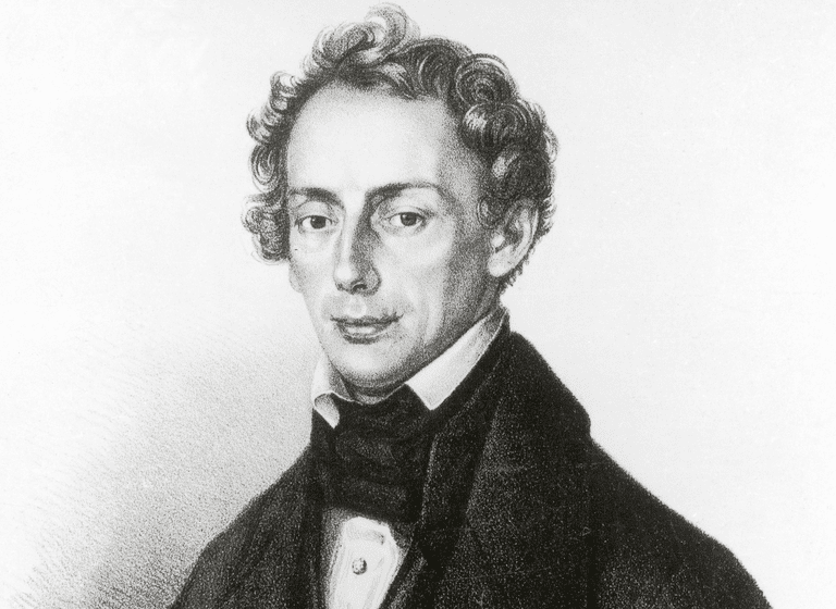
The irony of the Copernican system of the universe, when it was proposed in 1543 by Nicolaus Copernicus, is that it took stars that moved persistently through the heavens and fixed them in the sky, unmovable.  The “fixed stars” became the accepted norm for several centuries, until the peripatetic Edmund Halley (1656 – 1742) wondered if the stars really did not move.  From Newton’s new work on celestial dynamics (the famous Principia, which Halley generously paid out of his own pocket to have published not only because of his friendship with Newton, but because Halley believed it to be a monumental work that needed to be widely known), it was understood that gravitational effects would act on the stars and should cause them to move.

Fig. Halley’s Comet

In 1710 Halley began studying the accurate star-location records of Ptolemy from one and a half millennia earlier and compared  them with what he could see in the night sky.  He realized that the star Sirius had shifted in the sky by an angular distance equivalent to the diameter of the moon.  Other bright stars, like Arcturus and Procyon, also showed discrepancies from Ptolemy.  On the other hand, dimmer stars, that Halley reasoned were farther away, showed no discernible shifts in 1500 years.  At a time when stellar parallax, the apparent shift in star locations caused by the movement of the Earth, had not yet been detected, Halley had found an alternative way to get at least some ranked distances to the stars based on their proper motion through the universe.  Closer stars to the Earth would show larger angular displacements over 1500 years than stars farther away.  By being the closest bright star to Earth, Sirius had become a testbed for observations and theories of the motions of stars.  With the confidence of the confirmation of the nearness of Sirius to the Earth, Jacques Cassini claimed in 1714 to have measured the parallax of Sirius, but Halley refuted this claim in 1720.  Parallax would remain elusive for another hundred years to come.

The Sound of Sirius

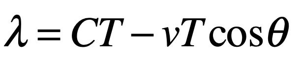
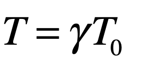
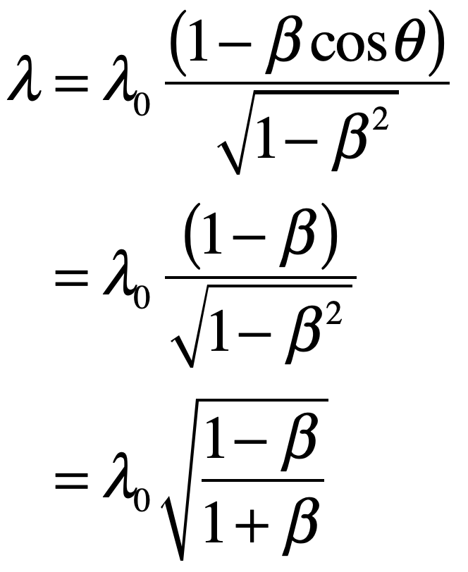
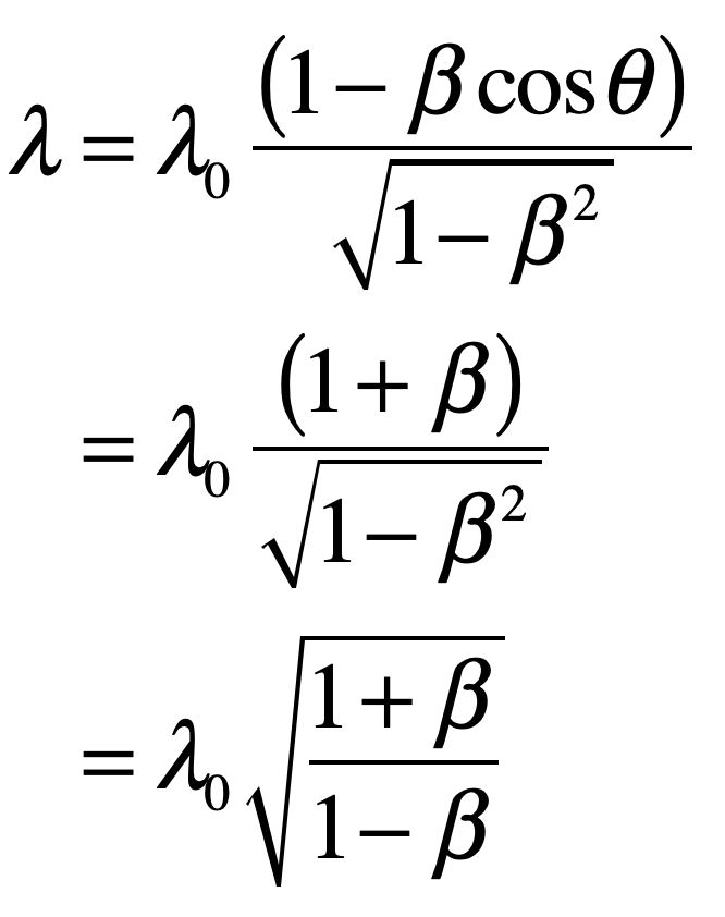
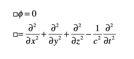
Of all the discoveries that emerged from nineteenth century physics—Young’s fringes, Biot-Savart law, Fresnel lens, Carnot cycle, Faraday effect, Maxwell’s equations, Michelson interferometer—only one is heard daily—the Doppler effect [1].  Doppler’s name is invoked every time you turn on the evening news to watch Doppler weather radar.  Doppler’s effect is experienced as you wait by the side of the road for a car to pass by or a jet to fly overhead.  Einstein may have the most famous name in physics, but Doppler’s is certainly the most commonly used.   

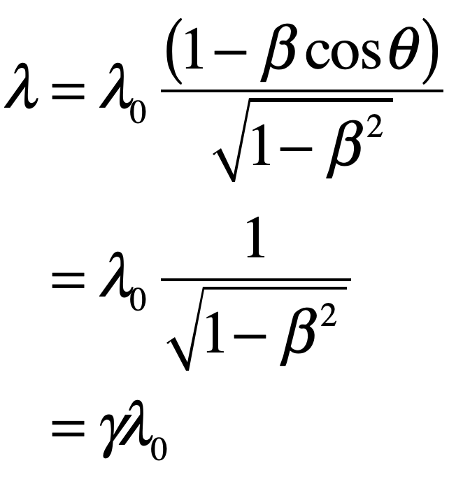
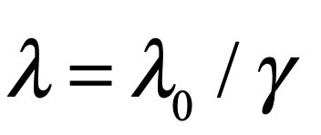
Although experimental support for the acoustic Doppler effect accumulated quickly, corresponding demonstrations of the optical Doppler effect were slow to emerge.  The breakthrough in the optical Doppler effect was made by William Huggins (1824-1910).  Huggins was an early pioneer in astronomical spectroscopy and was famous for having discovered that some bright nebulae consist of atomic gases (planetary nebula in our own galaxy) while others (later recognized as distant galaxies) consist of unresolved emitting stars.  Huggins was intrigued by the possibility of using the optical Doppler effect to measure the speed of stars, and he corresponded with James Clerk Maxwell (1831-1879) to confirm the soundness of Doppler’s arguments, which Maxwell corroborated using his new electromagnetic theory.  With the resulting confidence, Huggins turned his attention to the brightest star in the heavens, Sirius, and on May 14, 1868, he read a paper to the Royal Society of London claiming an observation of Doppler shifts in the spectral lines of the star Sirius consistent with a speed of about 50 km/sec [2].

Fig. Doppler spectroscopy of stellar absorption lines caused by the relative motion of the star (in this illustration the orbiting exoplanet is causing the star to wobble.)

The importance of Huggins’ report on the Doppler effect from Sirius was more psychological than scientifically accurate, because it convinced the scientific community that the optical Doppler effect existed.  Around this time the German astronomer Hermann Carl Vogel (1841 – 1907) of the Potsdam Observatory began working with a new spectrograph designed by Johann Zöllner from Leipzig [3] to improve the measurements of the radial velocity of stars (the speed along the line of sight).  He was aware that the many values quoted by Huggins and others for stellar velocities were nearly the same as the uncertainties in their measurements.  Vogel installed photographic capabilities in the telescope and spectrograph at the Potsdam Observatory [4] in 1887 and began making observations of Doppler line shifts in stars through 1890.  He published an initial progress report in 1891, and then a definitive paper in 1892 that provided the first accurate stellar radial velocities [5].  Fifty years after Doppler read his paper to the Royal Bohemian Society of Science (in 1842 to a paltry crowd of only a few scientists), the Doppler effect had become an established workhorse of quantitative astrophysics. A laboratory demonstration of the optical Doppler effect was finally achieved in 1901 by Aristarkh Belopolsky (1854-1934), a Russian astronomer, by constructing a device with a narrow-linewidth light source and rapidly rotating mirrors [6].

White Dwarf

While measuring the position of Sirius to unprecedented precision, the German astronomer Friedrich Wilhelm Bessel (1784 – 1846) noticed a slow shift in its position.  (This is the same Bessel as “Bessel function” fame, although the functions were originally developed by Daniel Bernoulli and Bessel later generalized them.)  Bessel deduced that Sirius must have an unseen companion with an orbital of around 50 years.  This companion was discovered by accident in 1862 during a test run of a new lens manufactured by the Clark&Sons glass manufacturing company prior to delivery to Northwestern University in Chicago.  (The lens was originally ordered by the University of Mississippi in 1860, but after the Civil War broke out, the Massachusetts-based Clark company put it up for bid.  Harvard wanted it, but Northwestern got it.)  Sirius itself was redesignated Sirius A, while this new star was designated Sirius B (and sometimes called “The Pup”). 

Fig. White dwarf and planet.

The Pup’s spectrum was measured in 1915 by Walter Adams (1876 – 1956) which put it in the newly-formed class of “white dwarf” stars that were very small but, unlike other types of dwarf stars, they had very hot (white) spectra.  The deflection of the orbit of Sirius A allowed its mass to be estimated at about one solar mass, which was normal for a dwarf star.  Furthermore, its brightness and surface temperature allowed its density to be estimated, but here an incredible number came out: the density of Sirius B was about 30,000 times greater than the density of the sun!  Astronomers at the time thought that this was impossible, and Arthur Eddington, who was the expert in star formation, called it “nonsense”.  This nonsense withstood all attempts to explain it for over a decade.

In 1926, R. H. Fowler (1889 – 1944) at Cambridge University in England applied the newly-developed theory of quantum mechanics and the Pauli exclusion principle to the problem of such ultra-dense matter.  He found that the Fermi sea of electrons provided a type of pressure, called degeneracy pressure, that counteracted the gravitational pressure that threatened to collapse the star under its own weight.  Several years later, Subrahmanyan Chandrasekhar calculated the upper limit for white dwarfs using relativistic effects and accurate density profiles and found that a white dwarf with a mass greater than about 1.5 times the mass of the sun would no longer be supported by the electron degeneracy pressure and would suffer gravitational collapse.  At the time, the question of what it would collapse to was unknown, although it was later understood that it would collapse to a neutron star.  Sirius B, at about one solar mass, is well within the stable range of white dwarfs.

But this was not the end of the story for Sirius B [7].  At around the time that Adams was measuring the spectrum of the white dwarf, Einstein was predicting that light emerging from a dense star would have its wavelengths gravitationally redshifted relative to its usual wavelength.  This was one of the three classic tests he proposed for his new theory of General Relativity.  (1 – The precession of the perihelion of Mercury. 2 – The deflection of light by gravity.  3 – The gravitational redshift of photons rising out of a gravity well.)  Adams announced in 1925 (after the deflection of light by gravity had been confirmed by Eddington in 1919) that he had measured the gravitational redshift.  Unfortunately, it was later surmised that he had not measured the gravitational effect but had actually measured Doppler-shifted spectra because of the rotational motion of the star.  The true gravitational redshift of Sirius B was finally measured in 1971, although the redshift of another white dwarf, 40 Eridani B, had already been measured in 1954.

Static Interference

The quantum nature of light is an elusive quality that requires second-order experiments of intensity fluctuations to elucidate them, rather than using average values of intensity.  But even in second-order experiments, the manifestations of quantum phenomenon are still subtle, as evidenced by an intense controversy that was launched by optical experiments performed in the 1950’s by a radio astronomer, Robert Hanbury Brown (1916 – 2002).  (For the full story, see Chapter 4 in my book Interference from Oxford (2023) [8]).

Hanbury Brown (he never went by his first name) was born in Aruvankandu, India, the son of a British army officer.  He never seemed destined for great things, receiving an unremarkable education that led to a degree in radio engineering from a technical college in 1935.  He hoped to get a PhD in radio technology, and he even received a scholarship to study at Imperial College in London, when he was urged by the rector of the university, Sir Henry Tizard, to give up his plans and join an effort to develop defensive radar against a growing threat from Nazi Germany as it aggressively rearmed after abandoning the punitive Versailles Treaty.  Hanbury Brown began the most exciting and unnerving five years of his life, right in the middle of the early development of radar defense, leading up to the crucial role it played in the Battle of Britain in 1940 and the Blitz from 1940 to 1941.  Partly due to the success of radar, Hitler halted night-time raids in the Spring of 1941, and England escaped invasion.

In 1949, fourteen years after he had originally planned to start his PhD, Hanbury Brown enrolled at the relatively ripe age of 33 at the University of Manchester.  Because of his background in radar, his faculty advisor told him to look into the new field of radio astronomy that was just getting started, and Manchester was a major player because it administrated the Jodrell Bank Observatory, which was one of the first and largest radio astronomy observatories in the World.  Hanbury Brown was soon applying all he had learned about radar transmitters and receivers to the new field, focusing particularly on aspects of radio interferometry after Martin Ryle (1918 – 1984) at Cambridge with Derek Vonberg (1921 – 2015) developed the first radio interferometer to measure the angular size of the sun [9] and of radio sources on the Sun’s surface that were related to sunspots [10].  Despite the success of their measurements, their small interferometer was unable to measure the size of other astronomical sources.  From Michelson’s formula for stellar interferometry, longer baselines between two separated receivers would be required to measure smaller angular sizes.  For his PhD project, Hanbury Brown was given the task of designing a radio interferometer to resolve the two strongest radio sources in the sky, Cygnus A and Cassiopeia A, whose angular sizes were unknown.  As he started the project, he was confronted with the problem of distributing a stable reference signal to receivers that might be very far apart, maybe even thousands of kilometers, a problem that had no easy solution. 

After grappling with this technical problem for months without success, late one night in 1949 Hanbury Brown had an epiphany [11], wondering what would happen if the two separate radio antennas measured only intensities rather than fields.  The intensity in a radio telescope fluctuates in time like random noise.  If that random noise were measured at two separated receivers while trained on a common source, would those noise patterns look the same?  After a few days considering this question, he convinced himself that the noise would indeed share common features, and the degree to which the two noise traces were similar should depend on the size of the source and the distance between the two receivers, just like Michelson’s fringe visibility.  But his arguments were back-of-the-envelope, so he set out to find someone with the mathematical skills to do it more rigorously.  He found Richard Twiss.

Richard Quentin Twiss (1920 – 2005), like Hanbury Brown, was born in India to British parents but had followed a more prestigious educational path, taking the Mathematical Tripos exam at Cambridge in 1941 and receiving his PhD from MIT in the United States in 1949.  He had just returned to England, joining the research division of the armed services located north of London, when he received a call from Hanbury Brown at the Jodrell Bank radio astronomy laboratory in Manchester.  Twiss travelled to meet Hanbury Brown in Manchester, who put him up in his flat in the neighboring town of Wilmslow.  The two set up the mathematical assumptions behind the new “intensity interferometer” and worked late into the night. When Hanbury Brown finally went to bed, Twiss was still figuring the numbers.  The next morning, the tall and lanky Twiss appeared in his silk dressing gown in the kitchen and told Hanbury Brown, “This idea of yours is no good, it doesn’t work”[12]—it would never be strong enough to detect the intensity from stars.  However, after haggling over the details of some of the integrals, Hanbury Brown, and then finally Twiss, became convinced that the effect was real.  Rather than fringe visibility, it was the correlation coefficient between two noise signals that would depend on the joint sizes of the source and receiver in a way that captured the same information as Michelson’s first-order fringe visibility.  But because no coherent reference wave was needed for interferometric mixing, this new approach could be carried out across very large baseline distances.

After demonstrating the effect on astronomical radio sources, Hanbury Brown and Twiss took the next obvious step: optical stellar intensity interferometry.  Their work had shown that photon noise correlations were analogous to Michelson fringe visibility, so the stellar intensity interferometer was expected to work similarly to the Michelson stellar interferometer—but with better stability over much longer baselines because it did not need a reference.  An additional advantage was the simple light collecting requirements.  Rather than needing a pair of massively expensive telescopes for high-resolution imaging, the intensity interferometer only needed to point two simple light collectors in a common direction.  For this purpose, and to save money, Hanbury Brown selected two of the largest army-surplus anti-aircraft searchlights that he could find left over from the London Blitz.  The lamps were removed and replaced with high-performance photomultipliers, and the units were installed on two train cars that could run along a railroad siding that crossed the Jodrell Bank grounds.

Fig. Stellar Interferometers: (Left) Michelson Stellar Field Interferometer. (Right) Hanbury Brown Twiss Stellar Intensity Interferometer.

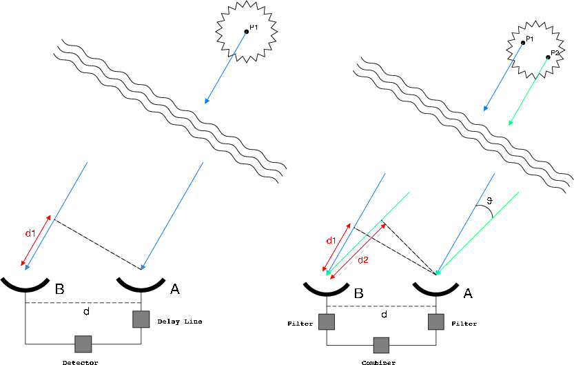
The target of the first test of the intensity interferometer was Sirius, the Dog Star.  Sirius was chosen because it is the brightest star in the night sky and was close to Earth at 8.6 light years and hence would be expected to have a relatively large angular size.  The observations began at the start of winter in 1955, but the legendary English weather proved an obstacle.  In addition to endless weeks of cloud cover, on many nights dew formed on the reflecting mirrors, making it necessary to install heaters.  It took more than three months to make 60 operational attempts to accumulate a mere 18 hours of observations [13].  But it worked!  The angular size of Sirius was measured for the first time. It subtended an angle of approximately 6 milliarcseconds (mas), which was well within the expected range for such a main sequence blue star.  This angle is equivalent to observing a house on the Moon from the Earth.  No single non-interferometric telescope on Earth, or in Earth orbit, has that kind of resolution, even today.  Once again, Sirus was the testbed of a new observational technology.  Hanbury Brown and Twiss went on the measure the diameters of dozens of stars.

Adaptive Optics

Any undergraduate optics student can tell you that bigger telescopes have higher spatial resolution.  But this is only true up to a point.  When telescope diameters become not much bigger than about 10 inches, the images they form start to dance, caused by thermal fluctuations in the atmosphere.  Large telescopes can still get “lucky” at moments when the atmosphere is quiet, but this usually only happens for a fraction of a second before the fluctuation set in again.  This is the primary reason that the Hubble Space Telescope was placed in Earth orbit above the atmosphere, and why the James Webb Space Telescope is flying a million miles away from the Earth.  But that is not the end of Earth-based large telescoped.  The Very Large Telescope (VLT) has a primary diameter of 8 meters, and the Extremely Large Telescope (ELT), coming online soon, has an even bigger diameter of 40 meters.  How do these work under the atmospheric blanket?  The answer is adaptive optics.

Adaptive optics uses active feedback to measure the dancing images caused by the atmosphere and uses the information to control a flexible array of mirror elements to exactly cancel out the effects of the atmospheric fluctuations.  In the early days of adaptive-optics development, the applications were more military than astronomic, but advances made in imaging enemy satellites soon was released to the astronomers.  The first civilian demonstrations of adaptive optics were performed in 1977 when researchers at Bell Labs [14] and at the Space Sciences Lab at UC Berkeley [15] each made astronomical demonstrations of improved seeing of the star Sirius using adaptive optics.  The field developed rapidly after that, but once again Sirius had led the way.

Star Travel

The day is fast approaching when humans will begin thinking seriously of visiting nearby stars—not in person at first, but with unmanned spacecraft that can telemeter information back to Earth.  Although Sirius is not the closest star to Earth—it is 8.6 lightyears away while Alpha Centauri is almost twice as close at only 4.2 lightyears away—it may be the best target for an unmanned spacecraft.  The reason is its brightness. 

Stardrive technology is still in its infancy—most of it is still on drawing boards.  Therefore, the only “mature” technology we have today is light pressure on solar sails.  Within the next 50 years or so we will have the technical ability to launch a solar sail towards a nearby star and accelerate it to a good fraction of the speed of light.  The problem is decelerating the spaceship when it arrives at its destination, otherwise it will go zipping by with only a few seconds to make measurements after its long trek there.

Fig. NASA’s solar sail demonstrator unit (artist’s rendering).

A better idea is to let the star light push against the solar sail to decelerate it to orbital speed by the time it arrives.  That way, the spaceship can orbit the target star for years.  This is a possibility with Sirius.  Because it is so bright, its light can decelerate the spaceship even when it is originally moving at relativistic speeds. By one calculation, the trip to Sirius, including the deceleration and orbital insertion, should only take about 69 years [16].  That’s just one lifetime.  Signals could be beaming back from Sirius by as early as 2100—within the lifetimes of today’s children.

By David D. Nolte, Sept. 4, 2024


Footnotes

[1] The section is excerpted from D. D. Nolte, The Fall and Rise of the Doppler Effect, Physics Today (2020)

[2] W. Huggins, “Further observations on the spectra of some of the stars and nebulae, with an attempt to determine therefrom whether these bodies are moving towards or from the earth, also observations on the spectra of the sun and of comet II,” Philos. Trans. R. Soc. London vol. 158, pp. 529-564, 1868. The correct value is -5.5 km/sec approaching Earth.  Huggins got the magnitude and even the sign wrong.

[3] in Hearnshaw, The Analysis of Starlight (Cambridge University Press, 2014), pg. 89

[4] The Potsdam Observatory was where the American Albert Michelson built his first interferometer while studying with Helmholtz in Berlin.

[5] Vogel, H. C. Publik. der astrophysik. Observ. Potsdam 1: 1. (1892)

[6] A. Belopolsky, “On an apparatus for the laboratory demonstration of the Doppler-Fizeau principle,” Astrophysical Journal, vol. 13, pp. 15-24, Jan 1901.

[7] https://adsabs.harvard.edu/full/1980QJRAS..21..246H

[8] D. D. Nolte, Interference: The History of Optical Interferometry and the Scientists who Tamed Light (Oxford University Press, 2023)

[9] M. Ryle and D. D. Vonberg, “Solar Radiation on 175 Mc/sec,” Nature, vol. 158 (1946): pp. 339-340.; K. I. Kellermann and J. M. Moran, “The development of high-resolution imaging in radio astronomy,” Annual Review of Astronomy and Astrophysics, vol. 39, (2001): pp. 457-509.

[10] M. Ryle, ” Solar radio emissions and sunspots,” Nature, vol. 161, no. 4082 (1948): pp. 136-136.

[11] R. H. Brown, The intensity interferometer; its application to astronomy (London, New York, Taylor & Francis; Halsted Press, 1974).

[12] R. H. Brown, Boffin : A personal story of the early days of radar and radio astronomy (Adam Hilger, 1991), p. 106.

[13] R. H. Brown and R. Q. Twiss. ” Test of a new type of stellar interferometer on Sirius.” Nature 178, no. 4541 (1956): pp. 1046-1048.

[14] S. L. McCall, T. R. Brown, and A. Passner, “IMPROVED OPTICAL STELLAR IMAGE USING A REAL-TIME PHASE-CORRECTION SYSTEM – INITIAL RESULTS,” Astrophysical Journal, vol. 211, no. 2, pp. 463-468, (1977)

[15] A. Buffington, F. S. Crawford, R. A. Muller, and C. D. Orth, “1ST OBSERVATORY RESULTS WITH AN IMAGE-SHARPENING TELESCOPE,” Journal of the Optical Society of America, vol. 67, no. 3, pp. 304-305, 1977 (1977)

[16] https://www.newscientist.com/article/2128443-quickest-we-could-visit-another-star-is-69-years-heres-how/


Read more in Books by David Nolte at Oxford University Press

The Doppler Universe

If you are a fan of the Doppler effect, then time trials at the Indy 500 Speedway will floor you.  Even if you have experienced the fall in pitch of a passing train whistle while stopped in your car at a railroad crossing, or heard the falling whine of a jet passing overhead, I can guarantee that you have never heard anything like an Indy car passing you by at 225 miles an hour.

Indy 500 Time Trials and the Doppler Effect

The Indy 500 time trials are the best way to experience the effect, rather than on race day when there is so much crowd noise and the overlapping sounds of all the cars.  During the week before the race, the cars go out on the track, one by one, in time trials to decide the starting order in the pack on race day.  Fans are allowed to wander around the entire complex, so you can get right up to the fence at track level on the straight-away.  The cars go by only thirty feet away, so they are coming almost straight at you as they approach and straight away from you as they leave.  The whine of the car as it approaches is 43% higher than when it is standing still, and it drops to 33% lower than the standing frequency—a ratio almost approaching a factor of two.  And they go past so fast, it is almost a step function, going from a steady high note to a steady low note in less than a second.  That is the Doppler effect!

But as obvious as the acoustic Doppler effect is to us today, it was far from obvious when it was proposed in 1842 by Christian Doppler at a time when trains, the fastest mode of transport at the time, ran at 20 miles per hour or less.  In fact, Doppler’s theory generated so much controversy that the Academy of Sciences of Vienna held a trial in 1853 to decide its merit—and Doppler lost!  For the surprising story of Doppler and the fate of his discovery, see my Physics Today article

From that fraught beginning, the effect has expanded in such importance, that today it is a daily part of our lives.  From Doppler weather radar, to speed traps on the highway, to ultrasound images of babies—Doppler is everywhere.

Development of the Doppler-Fizeau Effect

When Doppler proposed the shift in color of the light from stars in 1842 [1], depending on their motion towards or away from us, he may have been inspired by his walk to work every morning, watching the ripples on the surface of the Vltava River in Prague as the water slipped by the bridge piers.  The drawings in his early papers look reminiscently like the patterns you see with compressed ripples on the upstream side of the pier and stretched out on the downstream side.  Taking this principle to the night sky, Doppler envisioned that binary stars, where one companion was blue and the other was red, was caused by their relative motion.  He could not have known at that time that typical binary star speeds were too small to cause this effect, but his principle was far more general, applying to all wave phenomena. 

Six years later in 1848 [2], the French physicist Armand Hippolyte Fizeau, soon to be famous for making the first direct measurement of the speed of light, proposed the same principle, unaware of Doppler’s publications in German.  As Fizeau was preparing his famous measurement, he originally worked with a spinning mirror (he would ultimately use a toothed wheel instead) and was thinking about what effect the moving mirror might have on the reflected light.  He considered the effect of star motion on starlight, just as Doppler had, but realized that it was more likely that the speed of the star would affect the locations of the spectral lines rather than change the color.  This is in fact the correct argument, because a Doppler shift on the black-body spectrum of a white or yellow star shifts a bit of the infrared into the visible red portion, while shifting a bit of the ultraviolet out of the visible, so that the overall color of the star remains the same, but Fraunhofer lines would shift in the process.  Because of the independent development of the phenomenon by both Doppler and Fizeau, and because Fizeau was a bit clearer in the consequences, the effect is more accurately called the Doppler-Fizeau Effect, and in France sometimes only as the Fizeau Effect.  Here in the US, we tend to forget the contributions of Fizeau, and it is all Doppler.

Fig. 1 The title page of Doppler’s 1842 paper [1] proposing the shift in color of stars caused by their motions. (“On the colored light of double stars and a few other stars in the heavens: Study of an integral part of Bradley’s general aberration theory”)
Fig. 2 Doppler used simple proportionality and relative velocities to deduce the first-order change in frequency of waves caused by motion of the source relative to the receiver, or of the receiver relative to the source.
Fig. 3 Doppler’s drawing of what would later be called the Mach cone generating a shock wave. Mach was one of Doppler’s later champions, making dramatic laboratory demonstrations of the acoustic effect, even as skepticism persisted in accepting the phenomenon.

Doppler and Exoplanet Discovery

It is fitting that many of today’s applications of the Doppler effect are in astronomy. His original idea on binary star colors was wrong, but his idea that relative motion changes frequencies was right, and it has become one of the most powerful astrometric techniques in astronomy today. One of its important recent applications was in the discovery of extrasolar planets orbiting distant stars.

When a large planet like Jupiter orbits a star, the center of mass of the two-body system remains at a constant point, but the individual centers of mass of the planet and the star both orbit the common point. This makes it look like the star has a wobble, first moving towards our viewpoint on Earth, then moving away. Because of this relative motion of the star, the light can appear blueshifted caused by the Doppler effect, then redshifted with a set periodicity. This was observed by Queloz and Mayer in 1995 for the star 51 Pegasi, which represented the first detection of an exoplanet [3]. The duo won the Nobel Prize in 2019 for the discovery.

Fig. 4 A gas giant (like Jupiter) and a star obit a common center of mass causing the star to wobble. The light of the star when viewed at Earth is periodically red- and blue-shifted by the Doppler effect. From Ref.

Doppler and Vera Rubins’ Galaxy Velocity Curves

In the late 1960’s and early 1970’s Vera Rubin at the Carnegie Institution of Washington used newly developed spectrographs to use the Doppler effect to study the speeds of ionized hydrogen gas surrounding massive stars in individual galaxies [4]. From simple Newtonian dynamics it is well understood that the speed of stars as a function of distance from the galactic center should increase with increasing distance up to the average radius of the galaxy, and then should decrease at larger distances. This trend in speed as a function of radius is called a rotation curve. As Rubin constructed the rotation curves for many galaxies, the increase of speed with increasing radius at small radii emerged as a clear trend, but the stars farther out in the galaxies were all moving far too fast. In fact, they are moving so fast that they exceeded escape velocity and should have flown off into space long ago. This disturbing pattern was repeated consistently in one rotation curve after another for many galaxies.

Fig. 5 Locations of Doppler shifts of ionized hydrogen measured by Vera Rubin on the Andromeda galaxy. From Ref.
Fig. 6 Vera Rubin’s velocity curve for the Andromeda galaxy. From Ref.
Fig. 7 Measured velocity curves relative to what is expected from the visible mass distribution of the galaxy. From Ref.

A simple fix to the problem of the rotation curves is to assume that there is significant mass present in every galaxy that is not observable either as luminous matter or as interstellar dust. In other words, there is unobserved matter, dark matter, in all galaxies that keeps all their stars gravitationally bound. Estimates of the amount of dark matter needed to fix the velocity curves is about five times as much dark matter as observable matter. In short, 80% of the mass of a galaxy is not normal. It is neither a perturbation nor an artifact, but something fundamental and large. The discovery of the rotation curve anomaly by Rubin using the Doppler effect stands as one of the strongest evidence for the existence of dark matter.

There is so much dark matter in the Universe that it must have a major effect on the overall curvature of space-time according to Einstein’s field equations. One of the best probes of the large-scale structure of the Universe is the afterglow of the Big Bang, known as the cosmic microwave background (CMB).

Doppler and the Big Bang

The Big Bang was astronomically hot, but as the Universe expanded it cooled. About 380,000 years after the Big Bang, the Universe cooled sufficiently that the electron-proton plasma that filled space at that time condensed into hydrogen. Plasma is charged and opaque to photons, while hydrogen is neutral and transparent. Therefore, when the hydrogen condensed, the thermal photons suddenly flew free and have continued unimpeded, continuing to cool. Today the thermal glow has reached about three degrees above absolute zero. Photons in thermal equilibrium with this low temperature have an average wavelength of a few millimeters corresponding to microwave frequencies, which is why the afterglow of the Big Bang got its name: the Cosmic Microwave Background (CMB).

Not surprisingly, the CMB has no preferred reference frame, because every point in space is expanding relative to every other point in space. In other words, space itself is expanding. Yet soon after the CMB was discovered by Arno Penzias and Robert Wilson (for which they were awarded the Nobel Prize in Physics in 1978), an anisotropy was discovered in the background that had a dipole symmetry caused by the Doppler effect as the Solar System moves at 368±2 km/sec relative to the rest frame of the CMB. Our direction is towards galactic longitude 263.85o and latitude 48.25o, or a bit southwest of Virgo. Interestingly, the local group of about 100 galaxies, of which the Milky Way and Andromeda are the largest members, is moving at 627±22 km/sec in the direction of galactic longitude 276o and latitude 30o. Therefore, it seems like we are a bit slack in our speed compared to the rest of the local group. This is in part because we are being pulled towards Andromeda in roughly the opposite direction, but also because of the speed of the solar system in our Galaxy.

Fig. 8 The CMB dipole anisotropy caused by the Doppler effect as the Earth moves at 368 km/sec through the rest frame of the CMB.

Aside from the dipole anisotropy, the CMB is amazingly uniform when viewed from any direction in space, but not perfectly uniform. At the level of 0.005 percent, there are variations in the temperature depending on the location on the sky. These fluctuations in background temperature are called the CMB anisotropy, and they help interpret current models of the Universe. For instance, the average angular size of the fluctuations is related to the overall curvature of the Universe. This is because, in the early Universe, not all parts of it were in communication with each other. This set an original spatial size to thermal discrepancies. As the Universe continued to expand, the size of the regional variations expanded with it, and the sizes observed today would appear larger or smaller, depending on how the universe is curved. Therefore, to measure the energy density of the Universe, and hence to find its curvature, required measurements of the CMB temperature that were accurate to better than a part in 10,000.

Equivalently, parts of the early universe had greater mass density than others, causing the gravitational infall of matter towards these regions. Then, through the Doppler effect, light emitted (or scattered) by matter moving towards these regions contributes to the anisotropy. They contribute what are known as “Doppler peaks” in the spatial frequency spectrum of the CMB anisotropy.

Fig. 9 The CMB small-scale anisotropy, part of which is contributed by Doppler shifts of matter falling into denser regions in the early universe.

The examples discussed in this blog (exoplanet discovery, galaxy rotation curves, and cosmic background) are just a small sampling of the many ways that the Doppler effect is used in Astronomy. But clearly, Doppler has played a key role in the long history of the universe.

By David D. Nolte, Jan. 23, 2022


References:

[1] C. A. DOPPLER, “Über das farbige Licht der Doppelsterne und einiger anderer Gestirne des Himmels (About the coloured light of the binary stars and some other stars of the heavens),” Proceedings of the Royal Bohemian Society of Sciences, vol. V, no. 2, pp. 465–482, (Reissued 1903) (1842)

[2] H. Fizeau, “Acoustique et optique,” presented at the Société Philomathique de Paris, Paris, 1848.

[3] M. Mayor and D. Queloz, “A JUPITER-MASS COMPANION TO A SOLAR-TYPE STAR,” Nature, vol. 378, no. 6555, pp. 355-359, Nov (1995)

[4] Rubin, Vera; Ford, Jr., W. Kent (1970). “Rotation of the Andromeda Nebula from a Spectroscopic Survey of Emission Regions”. The Astrophysical Journal. 159: 379


Further Reading

D. D. Nolte, “The Fall and Rise of the Doppler Effect,” Physics Today, vol. 73, no. 3, pp. 31-35, Mar (2020)

M. Tegmark, “Doppler peaks and all that: CMB anisotropies and what they can tell us,” in International School of Physics Enrico Fermi Course 132 on Dark Matter in the Universe, Varenna, Italy, Jul 25-Aug 04 1995, vol. 132, in Proceedings of the International School of Physics Enrico Fermi, 1996, pp. 379-416

The Transverse Doppler Effect and Relativistic Time Dilation

One of the hardest aspects to grasp about relativity theory is the question of whether an event “looks as if” it is doing something, or whether it “actually is” doing something. 

Take, for instance, the classic twin paradox of relativity theory in which there are twins who wear identical high-precision wrist watches.  One of them rockets off to Alpha Centauri at relativistic speeds and returns while the other twin stays on Earth.  Each twin sees the other twin’s clock running slowly because of relativistic time dilation.  Yet when they get back together and, standing side-by-side, they compare their watches—the twin who went to Alpha Centauri is actually younger than the other, despite the paradox.  The relativistic effect of time dilation is “real”, not just apparent, regardless of whether they come back together to do the comparison.

Yet this understanding of relativistic effects took many years, even decades, to gain acceptance after Einstein proposed them.  He was aware himself that key experiments were required to prove that relativistic effects are real and not just apparent.

Einstein and the Transverse Doppler Effect

In 1905 Einstein used his new theory of special relativity to predict observable consequences that included relativistic velocity addition and a general treatment of the relativistic Doppler effect [1].  This included the effects of time dilation in addition to the longitudinal effect of the source chasing the wave.  Time dilation produced a correction to Doppler’s original expression for the longitudinal effect that became significant at speeds approaching the speed of light.  More significantly, it predicted a transverse Doppler effect for a source moving along a line perpendicular to the line of sight to an observer.  This effect had not been predicted either by Christian Doppler (1803 – 1853) or by Woldemar Voigt (1850 – 1919). 

( Read article in Physics Today on the history of the Doppler effect [2] )

Despite the generally positive reception of Einstein’s theory of special relativity, some of its consequences were anathema to many physicists at the time.  A key stumbling block was the question whether relativistic effects, like moving clocks running slowly, were only apparent, or were actually real, and Einstein had to fight to convince others of its reality.  When Johannes Stark (1874 – 1957) observed Doppler line shifts in ion beams called “canal rays” in 1906 (Stark received the 1919 Nobel prize in part for this discovery) [3], Einstein promptly published a paper suggesting how the canal rays could be used in a transverse geometry to directly detect time dilation through the transverse Doppler effect [4].  Thirty years passed before the experiment was performed with sufficient accuracy by Herbert Ives and G. R. Stilwell in 1938 to measure the transverse Doppler effect [5].  Ironically, even at this late date, Ives and Stilwell were convinced that their experiment had disproved Einstein’s time dilation by supporting Lorentz’ contraction theory of the electron.  The Ives-Stilwell experiment was the first direct test of time dilation, followed in 1940 by muon lifetime measurements [6].

A) Transverse Doppler Shift Relative to Emission Angle

The Doppler effect varies between blue shifts in the forward direction to red shifts in the backward direction, with a smooth variation in Doppler shift as a function of the emission angle.  Consider the configuration shown in Fig. 1 for light emitted from a source moving at speed v and emitting at an angle θ0 in the receiver frame. The source moves a distance vT in the time of a single emission cycle (assume a harmonic wave). In that time T (which is the period of oscillation of the light source — or the period of a clock if we think of it putting out light pulses) the light travels a distance cT before another cycle begins (or another pulse is emitted).

Fig. 1 Configuration for detection of Doppler shifts for emission angle θ0. The light source travels a distance vT during the time of a single cycle, while the wavefront travels a distance cT towards the detector.

[ See YouTube video on the derivation of the transverse Doppler Effect.]

The observed wavelength in the receiver frame is thus given by

where T is the emission period of the moving source.  Importantly, the emission period is time dilated relative to the proper emission time of the source

Therefore,

This expression can be evaluated for several special cases:

a) θ0 = 0 for forward emission

which is the relativistic blue shift for longitudinal motion in the direction of the receiver.

b) θ0 = π for backward emission

which is the relativistic red shift for longitudinal motion away from the receiver

c) θ0 = π/2 for transverse emission

This transverse Doppler effect for emission at right angles is a red shift, caused only by the time dilation of the moving light source.  This is the effect proposed by Einstein and observed by Stark that proved moving clocks tick slowly.  But it is not the only way to view the transverse Doppler effect.

B) Transverse Doppler Shift Relative to Angle at Reception

A different option for viewing the transverse Doppler effect is the angle to the moving source at the moment that the light is detected.  The geometry of this configuration relative to the previous is illustrated in Fig. 2.

Fig. 2 The detection point is drawn at a finite distance. However, the relationship between θ0 and θ1 is independent of the distance to the detector

The transverse distance to the detection point is

The length of the line connecting the detection point P with the location of the light source at the moment of detection is (using the law of cosines)

Combining with the first equation gives

An equivalent expression is obtained as

Note that this result, relating θ1 to θ0, is independent of the distance to the observation point.

When θ1 = π/2, then

yielding

for which the Doppler effect is

which is a blue shift.  This creates the unexpected result that sin θ0 = π/2 produces a red shift, while sin θ1 = π/2 produces a blue shift. The question could be asked: which one represents time dilation? In fact, it is sin θ0 = π/2 that produces time dilation exclusively, because in that configuration there is no foreshortening effect on the wavelength–only the emission time.

C) Compromise: The Null Transverse Doppler Shift

The previous two configurations each could be used as a definition for the transverse Doppler effect. But one gives a red shift and one gives a blue shift, which seems contradictory. Therefore, one might try to strike a compromise between these two cases so that sin θ1 = sin θ0, and the configuration is shown in Fig. 3.

This is the case when θ1 + θ2 = π.  The sines of the two angles are equal, yielding

and

which is solved for

Inserting this into the Doppler equation gives

where the Taylor’s expansion of the denominator (at low speed) cancels the numerator to give zero net Doppler shift. This compromise configuration represents the condition of null Doppler frequency shift. However, for speeds approaching the speed of light, the net effect is a lengthening of the wavelength, dominated by time dilation, causing a red shift.

D) Source in Circular Motion Around Receiver

An interesting twist can be added to the problem of the transverse Doppler effect: put the source or receiver into circular motion, one about the other. In the case of a source in circular motion around the receiver, it is easy to see that this looks just like case A) above for θ0 = π/2, which is the red shift caused by the time dilation of the moving source

However, there is the possible complication that the source is no longer in an inertial frame (it experiences angular acceleration) and therefore it is in the realm of general relativity instead of special relativity. In fact, it was Einstein’s solution to this problem that led him to propose the Equivalence Principle and make his first calculations on the deflection of light by gravity. His solution was to think of an infinite number of inertial frames, each of which was instantaneously co-moving with the same linear velocity as the source. These co-moving frames are inertial and can be analyzed using the principles of special relativity. The general relativistic effects come from slipping from one inertial co-moving frame to the next. But in the case of the circular transverse Doppler effect, each instantaneously co-moving frame has the exact configuration as case A) above, and so the wavelength is red shifted exactly by the time dilation.

Fig. Left: Moving source around a stationary receiver has red-shifted light (pure time dilation effect). Right. Moving receiver around a stationary source has blue-shifted light.

E) Receiver in Circular Motion Around Source

Now flip the situation and consider a moving receiver orbiting a stationary source.

With the notion of co-moving inertial frames now in hand, this configuration is exactly the same as case B) above, and the wavelength is blue shifted according to the equation

caused by foreshortening.

By David D. Nolte, June 3, 2021

New from Oxford Press: The History of Light and Interference (2023)

Read about the physics and history of light and optics.

References

[1] A. Einstein, “On the electrodynamics of moving bodies,” Annalen Der Physik, vol. 17, no. 10, pp. 891-921, Sep (1905)

[2] D. D. Nolte, “The Fall and Rise of the Doppler Effect,” Physics Today, vol. 73, no. 3, pp. 31-35, Mar (2020)

[3] J. Stark, W. Hermann, and S. Kinoshita, “The Doppler effect in the spectrum of mercury,” Annalen Der Physik, vol. 21, pp. 462-469, Nov 1906.

[4] A. Einstein, “Possibility of a new examination of the relativity principle,” Annalen Der Physik, vol. 23, no. 6, pp. 197-198, May (1907)

[5] H. E. Ives and G. R. Stilwell, “An experimental study of the rate of a moving atomic clock,” Journal of the Optical Society of America, vol. 28, p. 215, 1938.

[6] B. Rossi and D. B. Hall, “Variation of the Rate of Decay of Mesotrons with Momentum,” Physical Review, vol. 59, pp. 223–228, 1941.


Cancer Holography for Personalized Medicine

Imagine if you could use the physics of coherent light to record a 3D hologram of a cancer tumor and use it to select the best therapy for the cancer patient.

This week in Scientific Reports, a Nature Research publication, we demonstrate the first step towards that goal using dynamic speckle holography on patient cancer biopsies.

In a collaboration between Purdue University and the Northwestern University School of Medicine, we performed Doppler spectroscopy of intracellular dynamics of human epithelial ovarian cancer tumor biopsies and observed how they responded to selected anti-cancer drugs. Distinctly different Doppler spectra were observed for patients who went into remission versus those who failed to achieve cancer remission. This is the first clinical pilot trial of the technology, known as Biodynamic Imaging (BDI) that uses digital holography, published in human cancer research.

BDI may, in the future, make it possible to select the most effective therapies for individual cancer patients, realizing the long-sought dream of personalized cancer care.

Read it here: This latest research on personalized medicine has just been published with @SpringerNature in @ScientificReports.

The Purdue University Office of Technology Transfer has licensed the BDI patent portfolio to Animated Dynamics, Inc., located in Indianapolis, IN, that is working to commercialize the technology to translate it to the cancer clinic. Currently less than 40% of all cancer patients respond favorably to their chemotherapy. Using BDI technology our hope is to improve rates of remission in select cancer settings.

This work was supported by the NIH under the The Office of Physical Sciences – Oncology (OPSO) and by NSF CBET.

A Commotion in the Stars: The History of the Doppler Effect

Christian Andreas Doppler (1803 – 1853) was born in Salzburg, Austria, to a longstanding family of stonemasons.  As a second son, he was expected to help his older brother run the business, so his Father had him tested in his 18th year for his suitability for a career in business.  The examiner Simon Stampfer (1790 – 1864), an Austrian mathematician and inventor teaching at the Lyceum in Salzburg, discovered that Doppler had a gift for mathematics and was better suited for a scientific career.  Stampfer’s enthusiasm convinced Doppler’s father to enroll him in the Polytechnik Institute in Vienna (founded only a few years earlier in 1815) where he took classes in mathematics, mechanics and physics [1] from 1822 to 1825.  Doppler excelled in his courses, but was dissatisfied with the narrowness of the education, yearning for more breadth and depth in his studies and for more significance in his positions, feelings he would struggle with for his entire short life.  He left Vienna, returning to the Lyceum in Salzburg to round out his education with philosophy, languages and poetry.  Unfortunately, this four-year detour away from technical studies impeded his ability to gain a permanent technical position, so he began a temporary assistantship with a mathematics professor at Vienna.  As he approached his 30th birthday this term expired without prospects.  He was about to emigrate to America when he finally received an offer to teach at a secondary school in Prague.

To read about the attack by Joseph Petzval on Doppler’s effect and the effect it had on Doppler, see my feature article “The Fall and Rise of the Doppler Effect in Physics Today, 73(3) 30, March (2020).

Salzburg Austria

Doppler in Prague

Prague gave Doppler new life.  He was a professor with a position that allowed him to marry the daughter of a sliver and goldsmith from Salzburg.  He began to publish scholarly papers, and in 1837 was appointed supplementary professor of Higher Mathematics and Geometry at the Prague Technical Institute, promoted to full professor in 1841.  It was here that he met the unusual genius Bernard Bolzano (1781 – 1848), recently returned from political exile in the countryside.  Bolzano was a philosopher and mathematician who developed rigorous concepts of mathematical limits and is famous today for his part in the Bolzano-Weierstrass theorem in functional analysis, but he had been too liberal and too outspoken for the conservative Austrian regime and had been dismissed from the University in Prague in 1819.  He was forbidden to publish his work in Austrian journals, which is one reason why much of Bolzano’s groundbreaking work in functional analysis remained unknown during his lifetime.  However, he participated in the Bohemian Society for Science from a distance, recognizing the inventive tendencies in the newcomer Doppler and supporting him for membership in the Bohemian Society.  When Bolzano was allowed to return in 1842 to the Polytechnic Institute in Prague, he and Doppler became close friends as kindred spirits. 

Prague, Czech Republic

On May 25, 1842, Bolzano presided as chairman over a meeting of the Bohemian Society for Science on the day that Doppler read a landmark paper on the color of stars to a meagre assembly of only five regular members of the Society [2].  The turn-out was so small that the meeting may have been held in the robing room of the Society rather than in the meeting hall itself.  Leading up to this famous moment, Doppler’s interests were peripatetic, ranging widely over mathematical and physical topics, but he had lately become fascinated by astronomy and by the phenomenon of stellar aberration.  Stellar aberration was discovered by James Bradley in 1729 and explained as the result of the Earth’s yearly motion around the Sun, causing the apparent location of a distant star to change slightly depending on the direction of the Earth’s motion.  Bradley explained this in terms of the finite speed of light and was able to estimate it to within several percent [3].  As Doppler studied Bradley aberration, he wondered how the relative motion of the Earth would affect the color of the star.  By making a simple analogy of a ship traveling with, or against, a series of ocean waves, he concluded that the frequency of impact of the peaks and troughs of waves on the ship was no different than the arrival of peaks and troughs of the light waves impinging on the eye.  Because perceived color was related to the frequency of excitation in the eye, he concluded that the color of light would be slightly shifted to the blue if approaching, and to the red if receding from, the light source. 

Doppler wave fronts from a source emitting spherical waves moving with speeds β relative to the speed of the wave in the medium.

Doppler calculated the magnitude of the effect by taking a simple ratio of the speed of the observer relative to the speed of light.  What he found was that the speed of the Earth, though sufficient to cause the detectable aberration in the position of stars, was insufficient to produce a noticeable change in color.  However, his interest in astronomy had made him familiar with binary stars where the relative motion of the light source might be high enough to cause color shifts.  In fact, in the star catalogs there were examples of binary stars that had complementary red and blue colors.  Therefore, the title of his paper, published in the Proceedings of the Royal Bohemian Society of Sciences a few months after he read it to the society, was “On the Coloured Light of the Double Stars and Certain Other Stars of the Heavens: Attempt at a General Theory which Incorporates Bradley’s Theorem of Aberration as an Integral Part” [4]

Title page of Doppler’s 1842 paper introducing the Doppler Effect.

Doppler’s analogy was correct, but like all analogies not founded on physical law, it differed in detail from the true nature of the phenomenon.  By 1842 the transverse character of light waves had been thoroughly proven through the work of Fresnel and Arago several decades earlier, yet Doppler held onto the old-fashioned notion that light was composed of longitudinal waves.  Bolzano, fully versed in the transverse nature of light, kindly published a commentary shortly afterwards [5] showing how the transverse effect for light, and a longitudinal effect for sound, were both supported by Doppler’s idea.  Yet Doppler also did not know that speeds in visual binaries were too small to produce noticeable color effects to the unaided eye.  Finally, (and perhaps the greatest flaw in his argument on the color of stars) a continuous spectrum that extends from the visible into the infrared and ultraviolet would not change color because all the frequencies would shift together preserving the flat (white) spectrum.

The simple algebraic derivation of the Doppler Effect in the 1842 publication..

Doppler’s twelve years in Prague were intense.  He was consumed by his Society responsibilities and by an extremely heavy teaching load that included personal exams of hundreds of students.  The only time he could be creative was during the night while his wife and children slept.  Overworked and running on too little rest, his health already frail with the onset of tuberculosis, Doppler collapsed, and he was unable to continue at the Polytechnic.  In 1847 he transferred to the School of Mines and Forrestry in Schemnitz (modern Banská Štiavnica in Slovakia) with more pay and less work.  Yet the revolutions of 1848 swept across Europe, with student uprisings, barricades in the streets, and Hungarian liberation armies occupying the cities and universities, giving him no peace.  Providentially, his former mentor Stampfer retired from the Polytechnic in Vienna, and Doppler was called to fill the vacancy.

Although Doppler was named the Director of Austria’s first Institute of Physics and was elected to the National Academy, he ran afoul of one of the other Academy members, Joseph Petzval (1807 – 1891), who persecuted Doppler and his effect.  To read a detailed description of the attack by Petzval on Doppler’s effect and the effect it had on Doppler, see my feature article “The Fall and Rise of the Doppler Effect” in Physics Today, March issue (2020).

Christian Doppler

Voigt’s Transformation

It is difficult today to appreciate just how deeply engrained the reality of the luminiferous ether was in the psyche of the 19th century physicist.  The last of the classical physicists were reluctant even to adopt Maxwell’s electromagnetic theory for the explanation of optical phenomena, and as physicists inevitably were compelled to do so, some of their colleagues looked on with dismay and disappointment.  This was the situation for Woldemar Voigt (1850 – 1919) at the University of Göttingen, who was appointed as one of the first professors of physics there in 1883, to be succeeded in later years by Peter Debye and Max Born.  Voigt received his doctorate at the University of Königsberg under Franz Neumann, exploring the elastic properties of rock salt, and at Göttingen he spent a quarter century pursuing experimental and theoretical research into crystalline properties.  Voigt’s research, with students like Paul Drude, laid the foundation for the modern field of solid state physics.  His textbook Lehrbuch der Kristallphysik published in 1910 remained influential well into the 20th century because it adopted mathematical symmetry as a guiding principle of physics.  It was in the context of his studies of crystal elasticity that he introduced the word “tensor” into the language of physics.

At the January 1887 meeting of the Royal Society of Science at Göttingen, three months before Michelson and Morely began their reality-altering experiments at the Case Western Reserve University in Cleveland Ohio, Voit submitted a paper deriving the longitudinal optical Doppler effect in an incompressible medium.  He was responding to results published in 1886 by Michelson and Morely on their measurements of the Fresnel drag coefficient, which was the precursor to their later results on the absolute motion of the Earth through the ether. 

Fresnel drag is the effect of light propagating through a medium that is in motion.  The French physicist Francois Arago (1786 – 1853) in 1810 had attempted to observe the effects of corpuscles of light emitted from stars propagating with different speeds through the ether as the Earth spun on its axis and traveled around the sun.  He succeeded only in observing ordinary stellar aberration.  The absence of the effects of motion through the ether motivated Augustin-Jean Fresnel (1788 – 1827) to apply his newly-developed wave theory of light to explain the null results.  In 1818 Fresnel derived an expression for the dragging of light by a moving medium that explained the absence of effects in Arago’s observations.  For light propagating through a medium of refractive index n that is moving at a speed v, the resultant velocity of light is

where the last term in parenthesis is the Fresnel drag coefficient.  The Fresnel drag effect supported the idea of the ether by explaining why its effects could not be observed—a kind of Catch-22—but it also applied to light moving through a moving dielectric medium.  In 1851, Fizeau used an interferometer to measure the Fresnel drag coefficient for light moving through moving water, arriving at conclusions that directly confirmed the Fresnel drag effect.  The positive experiments of Fizeau, as well as the phenomenon of stellar aberration, would be extremely influential on the thoughts of Einstein as he developed his approach to special relativity in 1905.  They were also extremely influential to Michelson, Morley and Voigt.

 In his paper on the absence of the Fresnel drag effect in the first Michelson-Morley experiment, Voigt pointed out that an equation of the form

is invariant under the transformation

From our modern vantage point, we immediately recognize (to within a scale factor) the Lorentz transformation of relativity theory.  The first equation is common Galilean relativity, but the last equation was something new, introducing a position-dependent time as an observer moved with speed  relative to the speed of light [6].  Using these equations, Voigt was the first to derive the longitudinal (conventional) Doppler effect from relativistic effects.

Voigt’s derivation of the longitudinal Doppler effect used a classical approach that is still used today in Modern Physics textbooks to derive the Doppler effect.  The argument proceeds by considering a moving source that emits a continuous wave in the direction of motion.  Because the wave propagates at a finite speed, the moving source chases the leading edge of the wave front, catching up by a small amount by the time a single cycle of the wave has been emitted.  The resulting compressed oscillation represents a blue shift of the emitted light.  By using his transformations, Voigt arrived at the first relativistic expression for the shift in light frequency.  At low speeds, Voigt’s derivation reverted to Doppler’s original expression.

A few months after Voigt delivered his paper, Michelson and Morley announced the results of their interferometric measurements of the motion of the Earth through the ether—with their null results.  In retrospect, the Michelson-Morley experiment is viewed as one of the monumental assaults on the old classical physics, helping to launch the relativity revolution.  However, in its own day, it was little more than just another null result on the ether.  It did incite Fitzgerald and Lorentz to suggest that length of the arms of the interferometer contracted in the direction of motion, with the eventual emergence of the full Lorentz transformations by 1904—seventeen years after the Michelson results.

            In 1904 Einstein, working in relative isolation at the Swiss patent office, was surprisingly unaware of the latest advances in the physics of the ether.  He did not know about Voigt’s derivation of the relativistic Doppler effect  (1887) as he had not heard of Lorentz’s final version of relativistic coordinate transformations (1904).  His thinking about relativistic effects focused much farther into the past, to Bradley’s stellar aberration (1725) and Fizeau’s experiment of light propagating through moving water (1851).  Einstein proceeded on simple principles, unencumbered by the mental baggage of the day, and delivered his beautifully minimalist theory of special relativity in his famous paper of 1905 “On the Electrodynamics of Moving Bodies”, independently deriving the Lorentz coordinate transformations [7]

One of Einstein’s talents in theoretical physics was to predict new phenomena as a way to provide direct confirmation of a new theory.  This was how he later famously predicted the deflection of light by the Sun and the gravitational frequency shift of light.  In 1905 he used his new theory of special relativity to predict observable consequences that included a general treatment of the relativistic Doppler effect.  This included the effects of time dilation in addition to the longitudinal effect of the source chasing the wave.  Time dilation produced a correction to Doppler’s original expression for the longitudinal effect that became significant at speeds approaching the speed of light.  More significantly, it predicted a transverse Doppler effect for a source moving along a line perpendicular to the line of sight to an observer.  This effect had not been predicted either by Doppler or by Voigt.  The equation for the general Doppler effect for any observation angle is

Just as Doppler had been motivated by Bradley’s aberration of starlight when he conceived of his original principle for the longitudinal Doppler effect, Einstein combined the general Doppler effect with his results for the relativistic addition of velocities (also in his 1905 Annalen paper) as the conclusive treatment of stellar aberration nearly 200 years after Bradley first observed the effect.

Despite the generally positive reception of Einstein’s theory of special relativity, some of its consequences were anathema to many physicists at the time.  A key stumbling block was the question whether relativistic effects, like moving clocks running slowly, were only apparent, or were actually real, and Einstein had to fight to convince others of its reality.  When Johannes Stark (1874 – 1957) observed Doppler line shifts in ion beams called “canal rays” in 1906 (Stark received the 1919 Nobel prize in part for this discovery) [8], Einstein promptly published a paper suggesting how the canal rays could be used in a transverse geometry to directly detect time dilation through the transverse Doppler effect [9].  Thirty years passed before the experiment was performed with sufficient accuracy by Herbert Ives and G. R. Stilwell in 1938 to measure the transverse Doppler effect [10].  Ironically, even at this late date, Ives and Stilwell were convinced that their experiment had disproved Einstein’s time dilation by supporting Lorentz’ contraction theory of the electron.  The Ives-Stilwell experiment was the first direct test of time dilation, followed in 1940 by muon lifetime measurements [11].


Further Reading

D. D. Nolte, “The Fall and Rise of the Doppler Effect“, Phys. Today 73(3) pg. 30 (March, 2020)

D. D. Nolte, Interference: The History of Optical Interferometry and the Scientists who Tamed Light (Oxford University Press, 2023)


Notes

[1] pg. 15, Eden, A. (1992). The search for Christian Doppler. Wien, Springer-Verlag.

[2] pg. 30, Eden

[3] Bradley, J (1729). “Account of a new discoved Motion of the Fix’d Stars”. Phil Trans. 35: 637–660.

[4] C. A. DOPPLER, “Über das farbige Licht der Doppelsterne und einiger anderer Gestirne des Himmels (About the coloured light of the binary stars and some other stars of the heavens),” Proceedings of the Royal Bohemian Society of Sciences, vol. V, no. 2, pp. 465–482, (Reissued 1903) (1842).

[5] B. Bolzano, “Ein Paar Bemerkunen über die Neu Theorie in Herrn Professor Ch. Doppler’s Schrift “Über das farbige Licht der Doppersterne und eineger anderer Gestirnedes Himmels”,” Pogg. Anal. der Physik und Chemie, vol. 60, p. 83, 1843; B. Bolzano, “Christian Doppler’s neuste Leistunen af dem Gebiet der physikalischen Apparatenlehre, Akoustik, Optik and optische Astronomie,” Pogg. Anal. der Physik und Chemie, vol. 72, pp. 530-555, 1847.

[6] W. Voigt, “Uber das Doppler’sche Princip,” Göttinger Nachrichten, vol. 7, pp. 41–51, (1887). The common use of c to express the speed of light came later from Voigt’s student Paul Drude.

[7] A. Einstein, “On the electrodynamics of moving bodies,” Annalen Der Physik, vol. 17, pp. 891-921, 1905.

[8] J. Stark, W. Hermann, and S. Kinoshita, “The Doppler effect in the spectrum of mercury,” Annalen Der Physik, vol. 21, pp. 462-469, Nov 1906.

[9] A. Einstein, “”Über die Möglichkeit einer neuen Prüfung des Relativitätsprinzips”,” vol. 328, pp. 197–198, 1907.

[10] H. E. Ives and G. R. Stilwell, “An experimental study of the rate of a moving atomic clock,” Journal of the Optical Society of America, vol. 28, p. 215, 1938.

[11] B. Rossi and D. B. Hall, “Variation of the Rate of Decay of Mesotrons with Momentum,” Physical Review, vol. 59, pp. 223–228, 1941.