February 5, 2025September 3, 2025 by David D. Nolte

A Short History of Neural Networks

History of Dynamics
ai, Artificial Intelligence, Attention mechanism, convolutional neural network, Deep Learning, History of Physics, Hopfield network, Machine Learning, neural networks, Neurodynamics, Nonlinear Dynamics, recurrent neural network, technology, van der Pol oscillator
1 Comment

When it comes to questions about the human condition, the question of intelligence is at the top. What is the origin of our intelligence? How intelligent are we? And how intelligent can we make other things…things like artificial neural networks?

This is a short history of the science and technology of neural networks, not just artificial neural networks but also the natural, organic type, because theories of natural intelligence are at the core of theories of artificial intelligence. Without understanding our own intelligence, we probably have no hope of creating the artificial type.

Ramon y Cajal (1888): Visualizing Neurons

The story begins with Santiago Ramon y Cajal (1853 – 1934) who received the Nobel Prize in physiology in 1906 for his work illuminating natural neural networks. He built on work by Camillo Golgi, using a stain to give intracellular components contrast [1], and then went further to developed his own silver emulsions like those of early photography (which was one of his hobbies). Cajal was the first to show that neurons were individual constituents of neural matter and that their contacts were sequential: axons of sets of neurons contacted the dendrites of other sets of neurons, never axon-to-axon or dendrite-to-dendrite, to create a complex communication network. This became known as the neuron doctrine, and it is a central idea of neuroscience today.

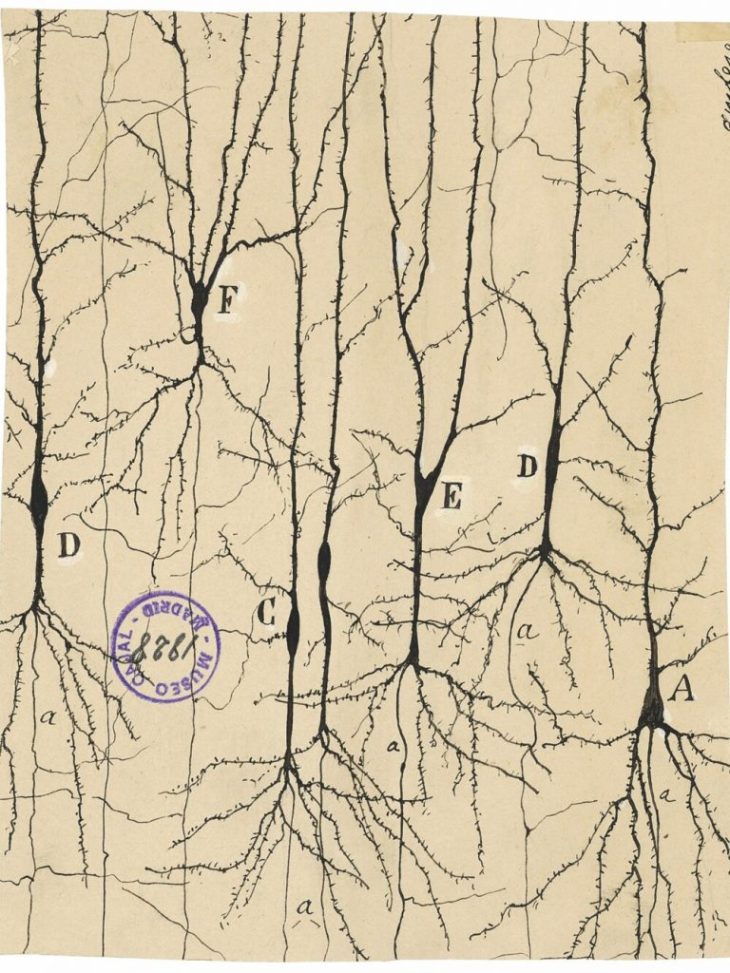
*Fig. 1 One of Cajal’s published plates demonstrating neural synapses. From Link.*

McCulloch and Pitts (1943): Mathematical Models

In 1941, Warren S. McCulloch (1898–1969) arrived at the Department of Psychiatry at the University of Illinois at Chicago where he met with the mathematical biology group at the University of Chicago led by Nicolas Rashevsky (1899–1972), widely acknowledged as the father of mathematical biophysics in the United States.

An itinerant member of Rashevsky’s group at the time was a brilliant, young and unusual mathematician, Walter Pitts (1923– 1969). He was not enrolled as a student at Chicago, but had simply “showed up” one day as a teenager at Rashevsky’s office door. Rashevsky was so impressed by Pitts that he invited him to attend the group meetings, and Pitts became interested in the application of mathematical logic to biological information systems.

When McCulloch met Pitts, he realized that Pitts had the mathematical background that complemented his own views of brain activity as computational processes. Pitts was homeless at the time, so McCulloch invited him to live with his family, giving the two men ample time to work together on their mutual obsession to provide a logical basis for brain activity in the way that Turing had provided it for computation.

McCulloch.and.Pitts Download

McColloch and Pitts simplified the operation of individual neurons to their most fundamental character, envisioning a neural computing unit with multiple inputs (received from upstream neurons) and a single on-off output (sent to downstream neurons) with the additional possibility of feedback loops as downstream neurons fed back onto upstream neurons. They also discretized the dynamics in time, using discrete logic and time-difference equations, succeeding in devising a logical structure with rules and equations for the general operation of nets of neurons. They published their results a 1943 in the paper titled “A logical calculus of the ideas immanent in nervous activity,” [2] introducing computational language and logic to neuroscience. Their simplified neural unit became the basis for discrete logic, picked up a few years later by von Neumann as an elemental example of a logic gate upon which von Neumann began constructing the theory and design of the modern electronic computer.

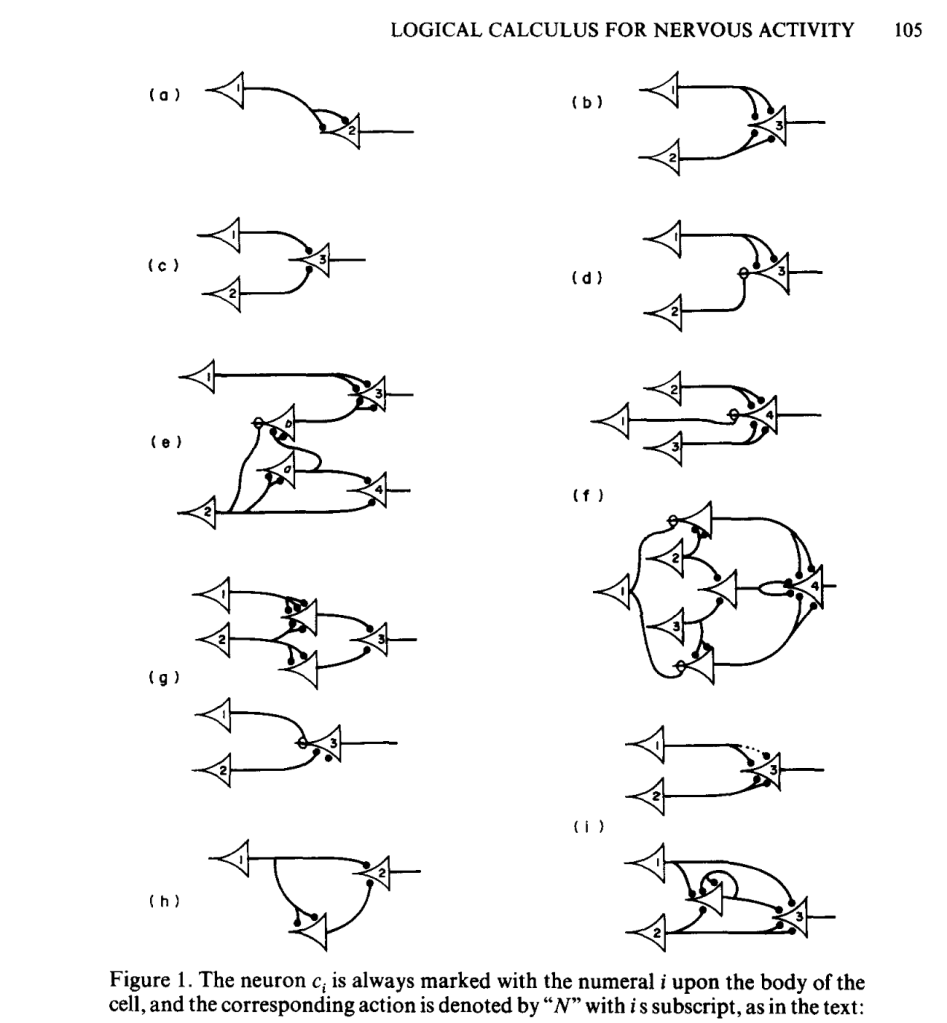
*Fig. 2 The only figure in McCulloch and Pitt’s “Logical Calculus”.*

Donald Hebb (1949): Hebbian Learning

The basic model for learning and adjustment of synaptic weights among neurons was put forward in 1949 by the physiological psychologist Donald Hebb (1904-1985) of McGill University in Canada in a book titled The Organization of Behavior [3].

In Hebbian learning, an initially untrained network consists of many neurons with many synapses having random synaptic weights. During learning, a synapse between two neurons is strengthened when both the pre-synaptic and post-synaptic neurons are firing simultaneously. In this model, it is essential that each neuron makes many synaptic contacts with other neurons because it requires many input neurons acting in concert to trigger the output neuron. In this way, synapses are strengthened when there is collective action among the neurons. The synaptic strengths are therefore altered through a form of self-organization. A collective response of the network strengthens all those synapses that are responsible for the response, while the other synapses that do not contribute, weaken. Despite the simplicity of this model, it has been surprisingly robust, standing up as a general principle for the training of artificial neural networks.

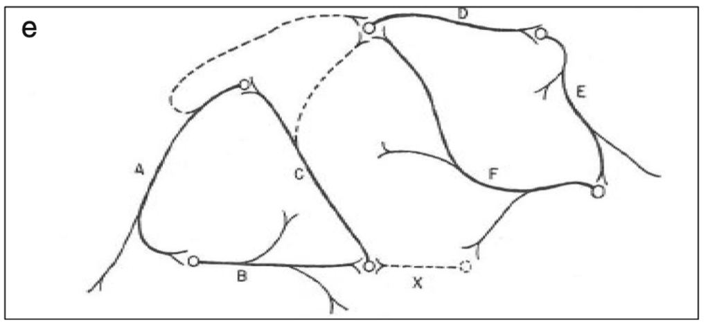
*Fig. 3. A Figure from Hebb’s textbook on psychology (1958). From Link.*

Hodgkin and Huxley (1952): Neuron Transporter Models

Alan Hodgkin (1914 – 1998) and Andrew Huxley (1917 – 2012) were English biophysicists who received the 1963 Nobel Prize in physiology for their work on the physics behind neural activation. They constructed a differential equation for the spiking action potential for which their biggest conceptual challenge was the presence of time delays in the voltage signals that were not explained by linear models of the neural conductance. As they began exploring nonlinear models, using their experiments to guide the choice of parameters, they settled on a dynamical model in a four-dimensional phase space. One dimension was voltage, while another was inhibitory current. The two remaining dimensions were sodium and potassium conductances, which they had determined were the major ions participating in the generation and propagation of the action potential. The nonlinear conductances of their model described the observed time delays and captured the essential neural behavior of the fast spike followed by a slow recovery. Huxley solved the equations on a hand-cranked calculator, taking over three months of tedious cranking to plot the numerical results.

*Fig. 4 The Hodgkin-Huxley model of the neuron, including capacitance C, voltage V and bias current I along with the conductances of potassium (K), sodium (Na) and Lithium (L) channels.*

Hodgkin and Huxley published [4] their measurements and their model (known as the Hodgkin-Huxley model) in a series of six papers in 1952 that led to an explosion of research in electrophysiology, for which Hodgkin and Huxley won the 1963 Nobel Prize in physiology or medicine. The four-dimensional Hodgkin–Huxley model stands as a classic example of the power of phenomenological modeling when combined with accurate experimental observation. Hodgkin and Huxley were able to ascertain not only the existence of ion channels in the cell membrane, but also their relative numbers, long before these molecular channels were ever directly observed using electron microscopes. The Hodgkin–Huxley model lent itself to simplifications that could capture the essential behavior of neurons while stripping off the details.

Frank Rosenblatt (1958): The Perceptron

Frank Rosenblatt (1928–1971) had a PhD in psychology from Cornell University and was in charge of the cognitive systems section of the Cornell Aeronautical Laboratory (CAL) located in Buffalo, New York. He was tasked with fulfilling a contract from the Navy to develop an analog image processor. Drawing from the work of McCulloch and Pitts, his team constructed a software system and then constructed a hardware model that adaptively updated the strength of the inputs, that they called neural weights, as it was trained on test images. The machine was dubbed the Mark I Perceptron, and its announcement in 1958 created a small media frenzy [5]. A New York Times article reported the perceptron was “the embryo of an electronic computer that [the navy] expects will be able to walk, talk, see, write, reproduce itself and be conscious of its existence.”

rosenblatt-1957 Download

The perceptron had a simple architecture, with two layers of neurons consisting of an input layer and a processing layer, and it was programmed by adjusting the synaptic weights to the inputs. This computing machine was the first to adaptively learn its functions, as opposed to following predetermined algorithms like digital computers. It seemed like a breakthrough in cognitive science and computing, as trumpeted by the New York Times. But within a decade, the development had stalled because the architecture was too restrictive.

Fig. 5 Frank Rosenblatt with his Perceptron. From Link.

Richard Fitzhugh and Jin-Ichi Nagumo (1961): Neural van der Pol Oscillators

In 1961 Richard FitzHugh (1922–2007), a neurophysiology researcher at the National Institute of Neurological Disease and Blindness (NINDB) of the National Institutes of Health (NIH), created a surprisingly simple model of the neuron that retained only a third order nonlinearity, just like the third-order nonlinearity that Rayleigh had proposed and solved in 1883, and that van der Pol extended in 1926. Around the same time that FitzHugh proposed his mathematical model [6], the electronics engineer Jin-Ichi Nagumo (1926-1999) in Japan created an electronic diode circuit with an equivalent circuit model that mimicked neural oscillations [7]. Together, this work by FitzHugh and Nagumo led to the so-called FitzHugh–Nagumo model. The conceptual importance of this model is that it demonstrated that the neuron was a self-oscillator, just like a violin string or wheel shimmy or the pacemaker cells of the heart. Once again, self-oscillators showed themselves to be common elements of a complex world—and especially of life.

*Fig. 6 The FitzHugh-Nagumo model of the neuron simplifies the Hodgkin-Huxley model from four dimensions down to two dimensions of voltage V and channel activation n.*

Fitzhugh_1961 Download

John Hopfield (1982): Spin Glasses and Recurrent Networks

John Hopfield (1933–) received his PhD from Cornell University in 1958, advised by Al Overhauser in solid state theory, and he continued to work on a broad range of topics in solid state physics as he wandered from appointment to appointment at Bell Labs, Berkeley, Princeton, and Cal Tech. In the 1970s Hopfield’s interests broadened into the field of biophysics, where he used his expertise in quantum tunneling to study quantum effects in biomolecules, and expanded further to include information transfer processes in DNA and RNA. In the early 1980s, he became aware of aspects of neural network research and was struck by the similarities between McColloch and Pitts’ idealized neuronal units and the physics of magnetism. For instance, there is a type of disordered magnetic material called a spin glass in which a large number of local regions of magnetism are randomly oriented. In the language of solid-state physics, one says that the potential energy function of a spin glass has a large number of local minima into which various magnetic configurations can be trapped. In the language of dynamics, one says that the dynamical system has a large number of basins of attraction [8].

Hopfieldpnas00447-0135 Download

The Parallel Distributed Processing Group (1986): Backpropagation

David Rumelhart, a mathematical psychologist at UC San Diego, was joined by James McClelland in 1974 and then by Geoffrey Hinton in 1978 to become what they called the Parallel Distributed Processing (PDP) group. The central tenets of the PDP framework they developed were: 1) processing is distributed across many semi-autonomous neural units, that 2) learn by adjusting the weights of their interconnections based on the strengths of their signals (i.e., Hebbian learning), whose memories and behaviors are 3) an emergent property of the distributed learned weights.

PDP was an exciting framework for artificial intelligence, and it captured the general behavior of natural neural networks, but it had a serious problem: How could all of the neural weights be trained?

In 1986, Rumelhart and Hinton with the mathematician Ronald Williams developed a mathematical procedure for training neural weights called error backpropagation [9]. The idea is actually very simple: create a mean squared error of the response of a neural network compared to an ideal response, then tweak one of the neural weights and see if the error increases or decreases. If the error decreases, keep the tweak for that weight and move to the next, working iteratively, tweak by tweak, to minimize the mean squared error. In this way, large numbers of neural weights can be adjusted as the network is trained to perform a specified task.

Error backpropagation has come a long way from that early 1986 paper, and it now lies at the core of the AI revolution we are experiencing today as tens of millions of neural weights are trained on massive datasets.

Rumelhart323533a0 Download

Yann LeCun (1989): Convolutional Neural Networks

In 1988, I was a new post-doc at AT&T Bell Labs at Holmdel, New Jersey fresh out of my PhD in physics from Berkeley. Bell Labs liked to give its incoming employees inspirational talks and tours of their facilities, and one of the tours I took was of the neural network lab run by Lawrence Jackel that was working on computer recognition of zip-code digits. The team’s new post-doc, arriving at Bell Labs the same time as me, was Yann LeCun. It is very possible that the demo our little group watched was run by him, or at least he was there, but at the time he was a nobody, so even if I had heard his name, it wouldn’t have meant anything to me.

Fast forward to today, and Yann LeCun’s name is almost synonomous with AI. He is the Chief AI Scientist at Facebook and his google scholar page reports that he gets 50,000 citations per year.

LeCun is famous for developing the convolutional neural network (CNN) in work that he published from Bell Labs in 1989 [10]. It is a biomimetic neural network that takes its inspiration from the receptive fields of the neural networks in the retina. What you think you see, when you look at something, is actually reconstructed by your brain. Your retina is a neural processor with receptive fields that are a far cry from one-to-one. Most prominent in the retina are center-surround fields, or kernels, that respond to the derivatives of the focused image instead of the image itself. It’s the derivatives that are sent up your optic neuron to your brain which then reconstructs the image. It works as a form of image compression so that broad uniform areas in an image are reduced to its edges.

LeCun.neco.1989.1.4.541 Download

The convolutional neural network works in the same way, it’s just engineered specifically to produce compressed and multiscale codes that capture broad areas as well as the fine details of an image. By constructing many different “kernel” operators at many different scales, it creates a set of features that capture the nuances of the image in quantitative form that is then processed by training neural weights in downstream neural networks.

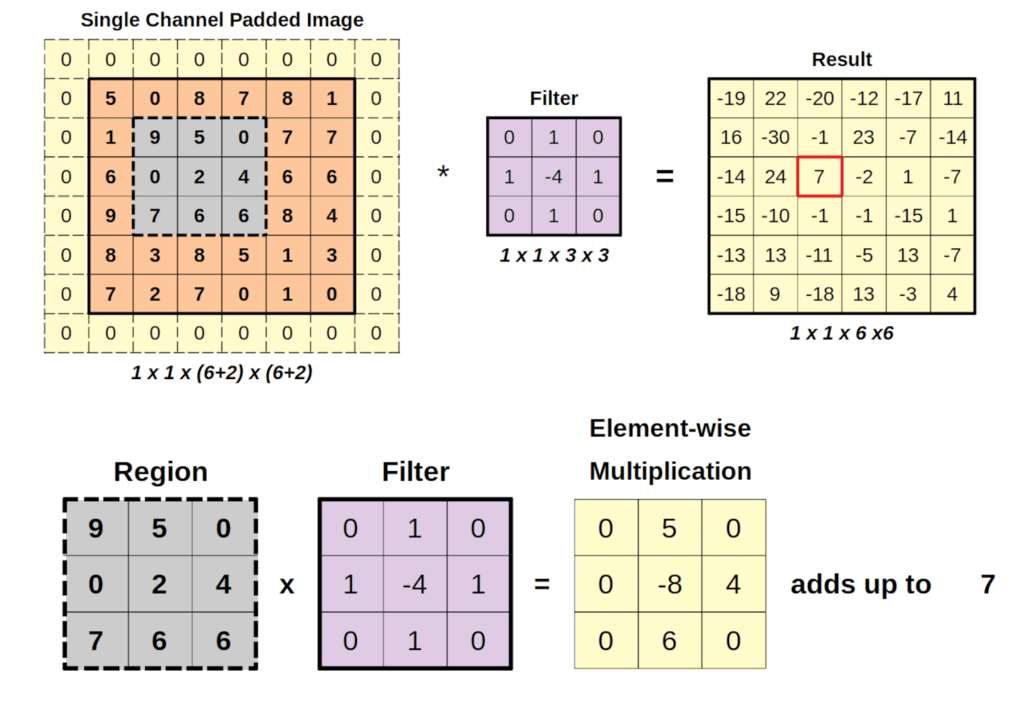
Fig. 7 Example of a receptive field of a CNN. The filter is the kernel (in this case a discrete 3×3 Laplace operator) that is stepped sequentially across the image field to produce the Laplacian feature map of the original image. One feature map for every different kernel becomes the input for the next level of kernels in a hierarchical scaling structure.

Geoff Hinton (2006): Deep Belief

It seems like Geoff Hinton has had his finger in almost every pie when it comes to how we do AI today. Backpropagation? Geoff Hinton. Rectified Linear Units? Geoff Hinton. Boltzmann Machines? Geoff Hinton. t-SNE? Geoff Hinton. Dropout regularization? Geoff Hinton. AlexNet? Geoff Hinton. The 2024 Nobel Prize in Physics? Geoff Hinton! He may not have invented all of these, but he was in the midst of it all.

Hinton received his PhD in Artificial Intelligence (ar rare field at the time) from the University of Edinburgh in 1978 after which he joined the PDP group at UCSD (see above) as a post-doc. After a time at Carnegie-Mellon, he joined the University of Toronto, Canada, in 1987 where he established one of the leading groups in the world on neural network research. It was from here that he launched so many of the ideas and techniques that have become the core of deep learning.

A central idea of deep learning came from Hinton’s work on Boltzmann Machines that learn statistical distributions of complex data. This type of neural network is known as an energy-based model, similar to a Hopfield network, and it has strong ties to the statistical mechanics of spin-glass systems. Unfortunately, it is a bitch to train! So Hinton simplified it into a Restricted Boltzmann Machine (RBM) that was much more tractable and layers of RBMs could be stacked into “Deep Belief Networks” [11] that had a hierarchical structure that allowed the neural nets to learn layers of abstractions. These were among the first deep networks that were able to do complex tasks at the level of human capabilities (and sometimes beyond).

The breakthrough that propelled Geoff Hinton to world-wide acclaim was the success of AlexNet, a neural network constructed by his graduate student Alex Krizhevsky at Toronto in 2012 consisting of 650,000 neurons with 60 million parameters that were trained using two early Nvidia GPUs. It won the ImageNet challenge that year, enabled by its deep architecture and representing a marked advancement that has been proceeding unabated today.

AttentionIsAllYouNeed2017 Download

Deep learning is now the rule in AI, supported by the Attention mechanism and Transformers that underpin the large language models, like ChatGPT and others, that are poised to disrupt all the legacy business models based on the previous silicon revolution of 50 years ago.

References

[1] Ramón y Cajal S. (1888). Estructura de los centros nerviosos de las aves. Rev. Trim. Histol. Norm. Pat. 1, 1–10.

[2] McCulloch, W.S. and W. Pitts, A Logical Calculus of the Ideas Immanent in Nervous Activity. Bull. Math. Biophys., 1943. 5: p. 115.

[3] Hebb, D. O. (1949). The Organization of Behavior: A Neuropsychological Theory. New York: Wiley and Sons. ISBN 978-0-471-36727-7 – via Internet Archive.

[4] Hodgkin AL, Huxley AF (August 1952). “A quantitative description of membrane current and its application to conduction and excitation in nerve”. The Journal of Physiology. 117 (4): 500–44.

[5] Rosenblatt, Frank (1957). “The Perceptron—a perceiving and recognizing automaton”. Report 85-460-1. Cornell Aeronautical Laboratory.

[6] FitzHugh, Richard (July 1961). “Impulses and Physiological States in Theoretical Models of Nerve Membrane”. Biophysical Journal. 1 (6): 445–466.

[7] Nagumo, J.; Arimoto, S.; Yoshizawa, S. (October 1962). “An Active Pulse Transmission Line Simulating Nerve Axon”. Proceedings of the IRE. 50 (10): 2061–2070.

[8] Hopfield, J. J. (1982). “Neural networks and physical systems with emergent collective computational abilities”. Proceedings of the National Academy of Sciences. 79 (8): 2554–2558.

[9] Rumelhart, D.E. et al. Nature 323, 533-536 (1986).

[10] Y. LeCun, B. Boser, J. S. Denker, D. Henderson, R. E. Howard, W. Hubbard and L. D. Jackel: Backpropagation Applied to Handwritten Zip Code Recognition, Neural Computation, 1(4):541–551, Winter 1989.

[11] G. E. Hinton, S. Osindero, and Y. W. Teh, “A fast learning algorithm for deep belief nets,” Neural Computation 18, 1527-1554 (2006).

Read more in Books by David D. Nolte at Oxford University Press

May 3, 2023September 5, 2025 by David D. Nolte

The Mighty Simplex

There is no greater geometric solid than the simplex. It is the paragon of efficiency, the pinnacle of symmetry, and the prototype of simplicity. If the universe were not constructed of continuous coordinates, then surely it would be tiled by tessellations of simplices.

Indeed, simplices, or simplexes, arise in a wide range of geometrical problems and real-world applications. For instance, metallic alloys are described on a simplex to identify the constituent elements [1]. Zero-sum games in game theory and ecosystems in population dynamics are described on simplexes [2], and the Dantzig simplex algorithm is a central algorithm for optimization in linear programming [3]. Simplexes also are used in nonlinear minimization (amoeba algorithm), in classification problems in machine learning, and they also raise their heads in quantum gravity. These applications reflect the special status of the simplex in the geometry of high dimensions.

… It’s Simplexes all the way down!

The reason for their usefulness is the simplicity of their construction that guarantees a primitive set that is always convex. For instance, in any space of d-dimensions, the simplest geometric figure that can be constructed of flat faces to enclose a d-volume consists of d+1 points that is the d-simplex.

Or …

In any space of d-dimensions, the simplex is the geometric figure whose faces are simplexes, whose faces are simplexes, whose faces are again simplexes, and those faces are once more simplexes … And so on.

In other words, it’s simplexes all the way down.

Simplex Geometry

In this blog, I will restrict the geometry to the regular simplex. The regular simplex is the queen of simplexes: it is the equilateral simplex for which all vertices are equivalent, and all faces are congruent, and all sub-faces are congruent, and so on. The regular simplexes have the highest symmetry properties of any polytope. A polytope is the d-dimensional generalization of a polyhedron. For instance, the regular 2-simplex is the equilateral triangle, and the regular 3-simplex is the equilateral tetrahedron.

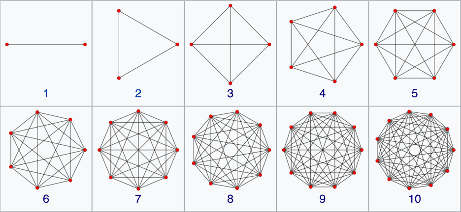
The N-simplex is the high-dimensional generalization of the tetrahedron. It is a regular N-dimensional polytope with N+1 vertexes. Starting at the bottom and going up, the simplexes are the point (0-simplex), the unit line (1-simplex), the equilateral triangle (2-simplex), the tetrahedron (3-simplex), the pentachoron (4-simplex), the hexateron (5-simplex) and onward. When drawn on the two-dimensional plane, the simplexes are complete graphs with links connecting every node to every other node. This dual character of equidistance and completeness give simplexes their utility. Each node is equivalent and is linked to each other. There are N•(N-1)/2 links among N vertices, and there are (N-2)•(N-1)/2 triangular faces.

Fig. 1 The N-simplex structures from 1-D through 10-D. Drawn on the 2D plane, the simplexes are complete graphs with links between every node. The number of vertices is equal to the number of dimensions plus one. (Wikipedia)

Fig. 2 Coulomb-spring visualization of the energy minimization of a 12-simplex (a 12-dimensional tetrahedron). Each node is a charge. Each link is a spring. Beginning as a complete graph on the planar circle, it finds a minimum configuration with 3 internal nodes.

Construction of a d-simplex is recursive: Begin with a (d-1)-dimensional simplex and add a point along an orthogonal dimension to construct a d-simplex. For instance, to create a 2-simplex (an equilateral triangle), find the mid-point of the 1-simplex (a line segment)

Centered 1-simplex: (-1), (1)

add a point on the perpendicular that is the same distance from each original vertex as the original vertices were distant from each other

Off-centered 2-simplex: (-1,0), (1,0), (0, sqrt(3)/2)

Then shift the origin to the center of mass of the triangle

Centered 2-simplex: (-1, -sqrt(3)/6), (1, -sqrt(3)/6), (0, sqrt(3)/3)

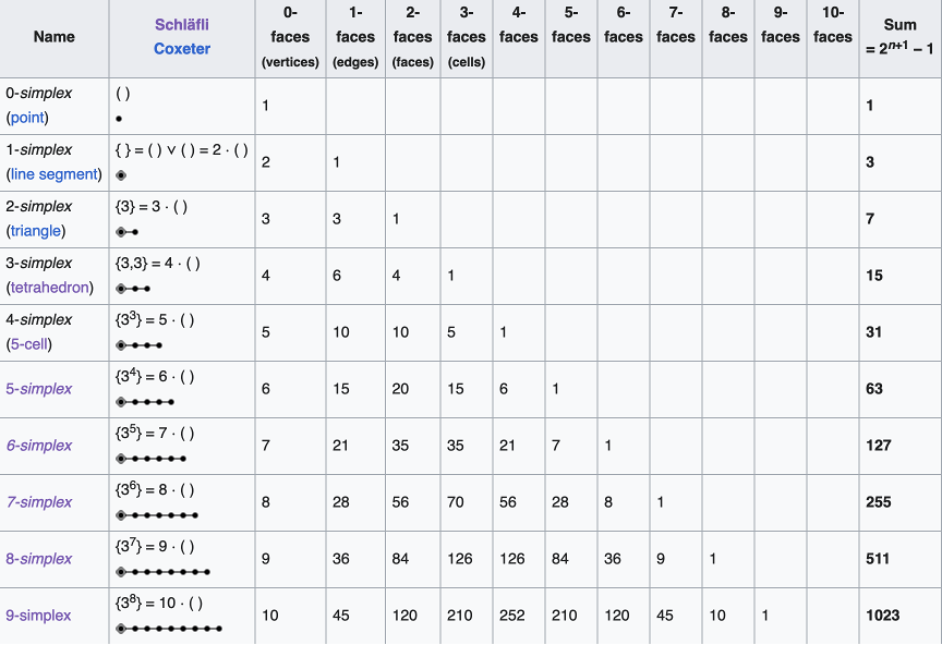
The 2-simplex, i.e., the equilateral triangle, has a 1-simplex as each of its faces. And each of those 1-simplexes has a 0-simplex as each of its ends. Therefore, this recursive construction of ever higher-dimensional simplexes out of low-dimensional ones, provides an interesting pattern:

*Fig. 3 The entries are the same numbers that appear in Pascal’s Triangle.* *(Wikipedia)*

The coordinates of an N-simplex are not unique, although there are several convenient conventions. One convention defines standard coordinates for an N-simplex in N+1 coordinate bases. These coordinates embed the simplex into a space of one higher dimension. For instance, the standard 2-simplex is defined by the coordinates (001), (010), (100) forming a two-dimensional triangle in three dimensions, and the simplex is a submanifold in the embedding space. A more efficient coordinate choice matches the coordinate-space dimensionality to the dimensionality of the simplex. Hence the 10 vertices of a 9-simplex can be defined by 9 coordinates (also not unique). One choice is given in Fig. 4 for the 1-simplex up to the 9-simplex.

*Fig. 4 One possible set of coordinates for the 1-simplex up to the 9-simplex. The center of mass of the simplex is at the origin, and the edge lengths are equal to 2.*

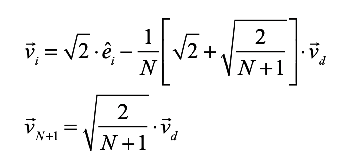
The equations for the simplex coordinates are

where

is the “diagonal” vector. These coordinates are centered on the center of mass of the simplex, and the links all have length equal to 2 which can be rescaled by a multiplying factor. The internal dihedral angle between all of the coordinate vectors for an N-simplex is

For moderate to high-dimensionality, the position vectors of the simplex vertices are pseudo-orthogonal. For instance, for N = 9 the dihedral angle cosine is -1/9 = -0.111. For higher dimensions, the simplex position vectors become asymptotically orthogonal. Such orthogonality is an important feature for orthonormal decomposition of class superpositions, for instance of overlapping images.

Alloy Mixtures and Barycentric Coordinates

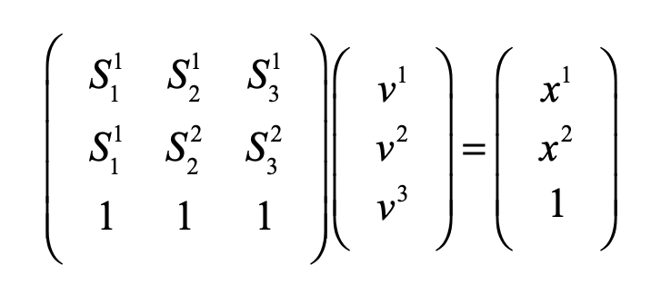
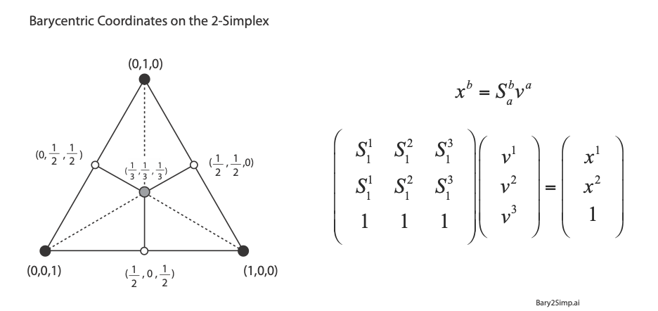
For linear systems, the orthonormality of basis representations is one of the most powerful features for system analysis in terms of superposition of normal modes. Neural networks, on the other hand, are intrinsically nonlinear decision systems for which linear superposition does not hold inside the network, even if the symbols presented to the network are orthonormal superpositions. This loss of orthonormality in deep networks can be partially retrieved by selecting the Simplex code. It has pseudo-orthogonal probability distribution functions located on the vertices of the simplex. There is an additional advantage to using the Simplex code: by using so-called barycentric coordinates, the simplex vertices can be expressed as independent bases. An example for the 2-simplex is shown in Fig. 5. The x-y Cartesian coordinates of the vertices (using tensor index notation) are given by (S₁¹, S₁²), (S₂¹, S₂²), and (S₃¹, S₃²). Any point (x¹, x²) on the plane can be expressed as a linear combination of the three vertices with barycentric coordinates (v¹, v², v³) by solving for these three coefficients from the equation

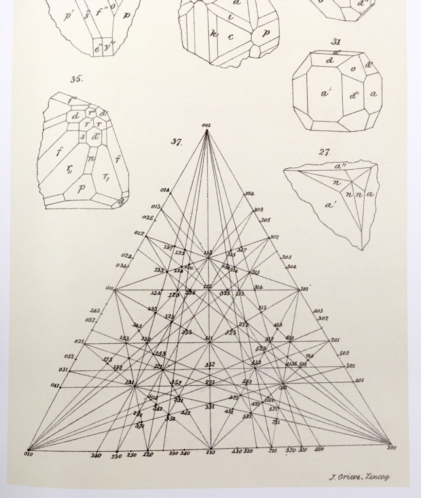
using Cramers rule. For instance, the three vertices of the simplex are expressed using the 3-component barycentric coordinates (1,0,0), (0,1,0) and (0,0,1). The mid-points on the edges have barycentric coordinates (1/2,1/2,0), (0,1/2,1/2), and (1/2,0,1/2). The centroid of the simplex has barycentric coordinates (1/3,1/3,1/3). Barycentric coordinates on a simplex are commonly used in phase diagrams of alloy systems in materials science. The simplex can also be used to identify crystallographic directions in three-dimensions, as in Fig. 6.

Fig. 5 Barycentric coordinates on the 2-Simplex. The vertices represent “orthogonal” pure symbols. Superpositions of 2 symbols lie on the edges. Any point on the simplex can be represented using barycentric coordinates with three indices corresponding to the mixture of the three symbols.

*Fig. 6 Crystallographic orientations expressed on a simplex. From A Treatise on Crystallography, William Miller, Cambridge (1839)*

Replicator Dynamics on the Simplex

Ecosystems are among the most complex systems on Earth. The complex interactions among hundreds or thousands of species may lead to steady homeostasis in some cases, to growth and collapse in other cases, and to oscillations or chaos in yet others. But the definition of species can be broad and abstract, referring to businesses and markets in economic ecosystems, or to cliches and acquaintances in social ecosystems, among many other examples. These systems are governed by the laws of evolutionary dynamics that include fitness and survival as well as adaptation. The dimensionality of the dynamical spaces for these systems extends to hundreds or thousands of dimensions—far too complex to visualize when thinking in four dimensions is already challenging.

A classic model of interacting species is the replicator equation. It allows for a fitness-based proliferation and for trade-offs among the individual species. The replicator dynamics equations are shown in Fig. 7.

Fig. 7 Replicator dynamics has a surprisingly simple form, but with surprisingly complicated behavior. The key elements are the fitness and the payoff matrix. The fitness relates to how likely the species will survive. The payoff matrix describes how one species gains at the loss of another (although symbiotic relationships also occur).

The population dynamics on the 2D simplex are shown in Fig. 8 for several different pay-off matrices (square matrix to the upper left of each simplex). The matrix values are shown in color and help interpret the trajectories. For instance the simplex on the upper-right shows a fixed point center. This reflects the antisymmetric character of the pay-off matrix around the diagonal. The stable spiral on the lower-left has a nearly asymmetric pay-off matrix, but with unequal off-diagonal magnitudes. The other two cases show central saddle points with stable fixed points on the boundary. A large variety of behaviors are possible for this very simple system. The Python program can be found in Trirep.py.

Fig. 8 Payoff matrix and population simplex for four random cases: Upper left is an unstable saddle. Upper right is a center. Lower left is a stable spiral. Lower right is a marginal case.

Linear Programming with the Dantzig Simplex

There is a large set of optimization problems in which a linear objective function is to be minimized subject to a set of inequalities. This is known as “Linear Programming”. These LP systems can be expressed as

The vector index goes from 1 to d, the dimension of the space. Each inequality creates a hyperplane, where two such hyperplanes intersect along a line terminated at each end by a vertex point. The set of vertexes defines a polytope in d-dimensions, and each face of the polytope, when combined with the point at the origin, defines a 3-simplex.

It is easy to visualize in lower dimensions why the linear objective function must have an absolute minimum at one of the vertexes of the polytope. And finding that minimum is a trivial exercise: Start at any vertex. Poll each neighboring vertex and move to the one that has the lowest value of the objective function. Repeat until the current vertex has a lower objective value than any neighbors. Because of the linearity of the objective function, this is a unique minimum (except for rare cases of accidental degeneracy). This iterative algorithm defines a walk on the vertexes of the polytope.

The question arises, why not just evaluate the objection function at each vertex and then just pick the vertex with the lowest value? The answer in high dimensions is that there are too many vertexes, and finding all of them is inefficient. If there are N vertexes, the walk to the solution visits only a few of the vertexes, on the order of log(N). The algorithm therefore scales as log(N), just like a search tree.

Fig. 9 Dantzig simplex approach on a convex 3D space of basic solutions in a linear programming problem.

This simple algorithm was devised by George Dantzig (1914 – 2005) in 1939 when he was a graduate student at UC Berkeley. He had arrived late to class and saw two problems written on the chalk board. He assumed that these were homework assignments, so he wrote them down and worked on them over the following week. He recalled that they seemed a bit harder than usual, but he eventually solved them and turned them in. A few weeks later, his very excited professor approached him and told him that the problems weren’t homework–they were two of the most important outstanding problems in optimization and that Dantzig had just solved them! The 1997 movie Good Will Hunting, with Matt Damon, Ben Affleck, and Robin Williams, borrowed this story for the opening scene.

The Amoeba Simplex Crawling through Hyperspace

Unlike linear programming problems with linear objective functions, multidimensional minimization of nonlinear objective functions is an art unto itself, with many approach. One of these is a visually compelling algorithm that does the trick more often than not. This is the so-called amoeba algorithm that shares much in common with the Dantzig simplex approach to linear programming, but instead of a set of fixed simplex coordinates, it uses a constantly shifting d-dimensional simplex that “crawls” over the objective function, seeking its minimum.

One of the best descriptions of the amoeba simplex algorithm is in “Numerical Recipes” [4] that describes the crawling simplex as

When it reaches a “valley floor”, the method contracts itself in the transverse direction and tries to ooze down the valley. If there is a situation where the simplex is trying to “pass through the eye of a needle”, it contracts itself in all directions, pulling itself in around its lowest (best) point.
(From Press, Numerical Recipes, Cambridge)

The basic operations for the crawling simplex are reflection and scaling. For a given evaluation of all the vertexes of the simplex, one will have the highest value and another the lowest. In a reflection, the highest point is reflected through the d-dimensional face defined by the other d vertexes. After reflection, if the new evaluation is lower than the former lowest value, then the point is expanded. If, on the other hand, it is little better than it was before reflection, then the point is contracted. The expansion and contraction are what allows the algorithm to slide through valleys or shrink to pass through the eye of a needle.

The amoeba algorithm was developed by John Nelder and Roger Mead in 1965 at a time when computing power was very limited. The algorithm works great as a first pass at a minimization problem, and it almost always works for moderately small dimensions, but for very high dimensions there are more powerful algorithms today for optimization, built into all the deep learning software environments like Tensor Flow and the Matlab toolbox.

By David D. Nolte, May 3, 2023

[1] M. Hillert, Phase equilibria, phase diagrams and phase transformations : their thermodynamic basis. (Cambridge University Press, Cambridge, UK ;, ed. 2nd ed., 2008).

[2] P. Schuster, K. Sigmund, Replicator Dynamics. Journal of Theoretical Biology 100, 533-538 (1983); P. Godfrey-Smith, The replicator in retrospect. Biology & Philosophy 15, 403-423 (2000).

[3] R. E. Stone, C. A. Tovey, The Simplex and Projective Scaling Algorithms as Iteratively Reweighted Least-squares Methods. Siam Review 33, 220-237 (1991).

[4] W. H. Press, Numerical Recipes in C++ : The Art of Scientific Computing. (Cambridge University Press, Cambridge, UK; 2nd ed., 2002).

Read more in Books by David Nolte at Oxford University Press

April 18, 2022February 9, 2023 by David D. Nolte

Post-Modern Machine Learning: The Deep Revolution

The mysteries of human intelligence are among the final frontiers of science. Despite our pride in what science has achieved across the past century, we have stalled when it comes to understanding intelligence or emulating it. The best we have done so far is through machine learning — harnessing the computational power of computers to begin to mimic the mind, attempting to answer the essential question:

How do we get machines to Know what we Know?

In modern machine learning, the answer is algorithmic.

In post-modern machine learning, the answer is manifestation.

The algorithms of modern machine learning are cause and effect, rules to follow, producing only what the programmer can imagine. But post-modern machine learning has blown past explicit algorithms to embrace deep networks. Deep networks today are defined by neural networks with thousands, or tens of thousands, or even hundreds of thousands, of neurons arrayed in multiple layers of dense connections. The interactivity of so many crossing streams of information defies direct deconstruction of what the networks are doing — they are post-modern. Their outputs manifest themselves, self-assembling into simplified structures and patterns and dependencies that are otherwise buried unseen in complicated data.

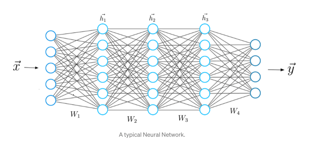
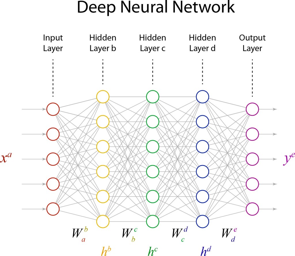
Fig. 1 A representation of a deep network with three fully-connected hidden layers. Deep networks are typically three or more layers deep, but each layer can have thousands of neurons. (Figure from the TowardsDataScience blog.)

Deep learning emerged as recently as 2006 and has opened wide new avenues of artificial intelligence that move beyond human capabilities for some tasks. But deep learning also has pitfalls, some of which are inherited from the legacy approaches of traditional machine learning, and some of which are inherent in the massively high-dimensional spaces in which deep learning takes place. Nonetheless, deep learning has revolutionized many aspects of science, and there is reason for optimism that the revolution will continue. Fifty years from now, looking back, we may recognize this as the fifth derivative of the industrial revolution (Phase I: Steam. Phase II: Electricity. Phase III: Automation. Phase IV: Information. Phase V: Intelligence).

From Multivariate Analysis to Deep Learning

Conventional machine learning, as we know it today, has had many names. It began with Multivariate Analysis of mathematical population dynamics around the turn of the last century, pioneered by Francis Galton (1874), Karl Pearson (1901), Charles Spearman (1904) and Ronald Fisher (1922) among others.

The first on-line computers during World War II were developed to quickly calculate the trajectories of enemy aircraft for gunnery control, introducing the idea of feedback control of machines. This was named Cybernetics by Norbert Wiener, who had participated in the development of automated control of antiaircraft guns.

Table I. Evolution of Names for Machine Learning

Multivariate Analysis (early-to-mid 1900’s)
Cybernetics (1940’s – 1950’s)
Connectionism (1960’s – 1970’s)
Parallel Distributed Processing (1970’s – 1980’s)
Neural Networks (1980’s – 1990’s)
Deep Learning (2000’s – today)

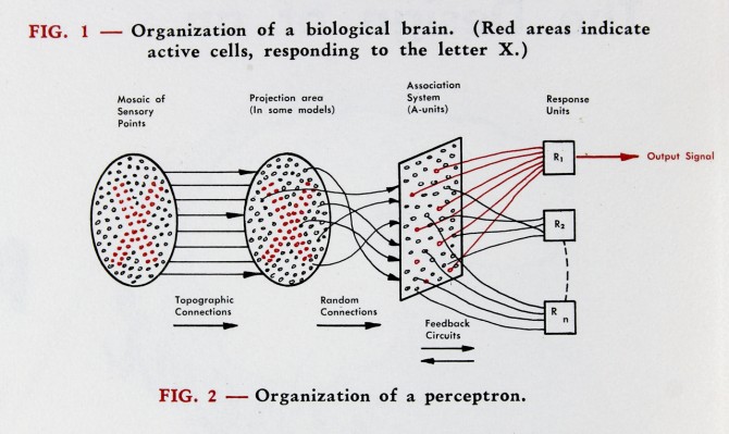
A decade later, during the Cold War, it became necessary to find hidden objects in large numbers of photographs. The embryonic electronic digital computers of the day were far too slow with far too little memory to do the task, so the Navy contracted with the Cornell Aeronautical Laboratory in Cheektowaga, New York, a suburb of Buffalo, to create an analog computer capable of real-time image analysis. This led to the invention of the Perceptron by Frank Rosenblatt as the first neural network-inspired computer [1], building on ideas of neural logic developed by Warren McColloch and Walter Pitts.

Fig. 2 Frank Rosenblatt working on the Perceptron. (From the Cornell Chronicle)

Fig. 3 Rosenblatt’s conceptual design of the connectionism of the perceptron (1958).

Several decades passed with fits and starts as neural networks remained too simple to accomplish anything profound. Then in 1986, David Rumelhart and Ronald Williams at UC San Diego with Geoff Hinton at Carnegie-Mellon discovered a way to train multiple layers of neurons, in a process called error back propagation [2]. This publication opened the floodgates of Connectionism — also known as Parallel Distributed Processing. The late 80’s and much of the 90’s saw an expansion of interest in neural networks, until the increasing size of the networks ran into limits caused by the processing speed and capacity of conventional computers towards the end of the decade. During this time it had become clear that the most interesting computations required many layers of many neurons, and the number of neurons expanded into the thousands, but it was difficult to train such systems that had tens of thousands of adjustable parameters, and research in neural networks once again went into a lull.

The beginnings of deep learning started with two breakthroughs. The first was by Yann Lecun at Bell Labs in 1998 who developed, with Leon Bottou, Yoshua Bengio and Patrick Haffner, a Convolutional Neural Network that had seven layers of neurons that classified hand-written digits [3]. The second was from Geoff Hinton in 2006, by then at the University of Toronto, who discovered a fast learning algorithm for training deep layers of neurons [4]. By the mid 2010’s, research on neural networks was hotter than ever, propelled in part by several very public successes, such as Deep Mind’s machine that beat the best player in the world at Go in 2017, self-driving cars, personal assistants like Siri and Alexa, and YouTube recommendations.

The Challenges of Deep Learning

Deep learning today is characterized by neural network architectures composed of many layers of many neurons. The nature of deep learning brings with it two main challenges: 1) efficient training of the neural weights, and 2) generalization of trained networks to perform accurately on previously unseen data inputs.

Solutions to the first challenge, efficient training, are what allowed the deep revolution in the first place—the result of a combination of increasing computer power with improvements in numerical optimization. This included faster personal computers that allowed nonspecialists to work with deep network programming environments like Matlab’s Deep Learning toolbox and Python’s TensorFlow.

Solutions to the second challenge, generalization, rely heavily on a process known as “regularization”. The term “regularization” has a slippery definition, an obscure history, and an awkward sound to it. Regularization is the noun form of the verb “to regularize” or “to make regular”. Originally, regularization was used to keep certain inverse algorithms from blowing up, like inverse convolutions, also known as deconvolution. Direct convolution is a simple mathematical procedure that “blurs” ideal data based on the natural response of a measuring system. However, if one has experimental data, one might want to deconvolve the system response from the data to recover the ideal data. But this procedure is numerically unstable and can “blow up”, often because of the divide-by-zero problem. Regularization was a simple technique that kept denominators from going to zero.

Regularization became a common method for inverse problems that are notorious to solve because of the many-to-one mapping that can occur in measurement systems. There can be a number of possible causes that produce a single response. Regularization was a way of winnowing out “unphysical” solutions so that the physical inverse solution remained.

During the same time, regularization became a common tool used by quantum field theorists to prevent certain calculated quantities from diverging to infinity. The solution was again to keep denominators from going to zero by setting physical cut-off lengths on the calculations. These cut-offs were initially ad hoc, but the development of renormalization group theory by Kenneth Wilson at Cornell (Nobel Prize in 1982) provided a systematic approach to solving the infinities of quantum field theory.

With the advent of neural networks, having hundreds to thousands to millions of adjustable parameters, regularization became the catch-all term for fighting the problem of over-fitting. Over-fitting occurs when there are so many adjustable parameters that any training data can be fit, and the neural network becomes just a look-up table. Look-up tables are the ultimate hash code, but they have no predictive capability. If a slightly different set of data are fed into the network, the output can be anything. In over-fitting, there is no generalization, the network simply learns the idiosyncrasies of the training data without “learning” the deeper trends or patterns that would allow it to generalize to handle different inputs.

Over the past decades a wide collection of techniques have been developed to reduce over-fitting of neural networks. These techniques include early stopping, k-fold holdout, drop-out, L1 and L2 weight-constraint regularization, as well as physics-based constraints. The goal of all of these techniques is to keep neural nets from creating look-up tables and instead learning the deep codependencies that exist within complicated data.

Table II. Regularization Techniques in Machine Learning

By judicious application of these techniques, combined with appropriate choices of network design, amazingly complex problems can be solved by deep networks and they can generalized too (to some degree). As the field moves forward, we may expect additional regularization tricks to improve generalization, and design principles will emerge so that the networks no longer need to be constructed by trial and error.

The Potential of Deep Learning

In conventional machine learning, one of the most critical first steps performed on a dataset has been feature extraction. This step is complicated and difficult, especially when the signal is buried either in noise or in confounding factors (also known as distractors). The analysis is often highly sensitive to the choice of features, and the selected features may not even be the right ones, leading to bad generalization. In deep learning, feature extraction disappears into the net itself. Optimizing the neural weights subject to appropriate constraints forces the network to find where the relevant information lies and what to do with it.

The key to finding the right information was not just having many neurons, but having many layers, which is where the potential of deep learning emerges. It is as if each successive layer is learning a more abstract or more generalized form of the information than the last. This hierarchical layering is most evident in the construction of convolutional deep networks, where the layers are receiving a telescoping succession of information fields from lower levels. Geoff Hinton‘s Deep Belief Network, which launched the deep revolution in 2006, worked explicitly with this hierarchy in mind through direct design of the network architecture. Since then, network architecture has become more generalized, with less up-front design while relying on the increasingly sophisticated optimization techniques of training to set the neural weights. For instance, a simplified instance of a deep network is shown in Fig. 4 with three hidden layers of neurons.

Fig. 4 General structure of a deep network with three hidden layers. Layers will typically have hundreds or thousands of neurons. Each gray line represents a weight value, and each circle is a neural activation function.

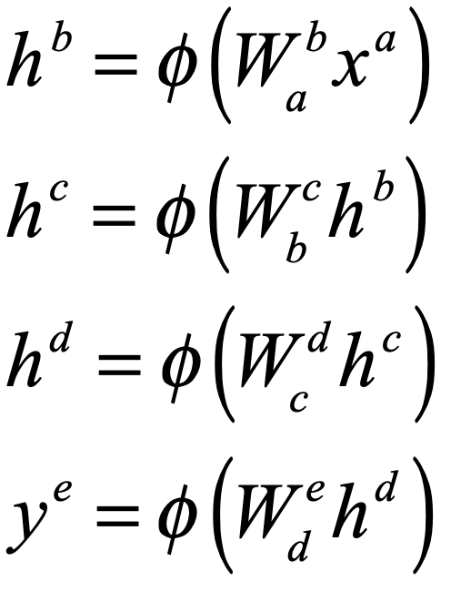
The mathematical structure of a deep network is surprisingly simple. The equations for the network in Fig. 4, that convert an input x^a to an output y^e, are

These equations use index notation to denote vectors (single superscript) and matrices (double indexes). The repeated index (one up and one down) denotes an implicit “Einstein” summation. The function φ(.) is known as the activation function, which is nonlinear. One of the simplest activation functions to use and analyze, and the current favorite, is known as the ReLU (for rectifying linear unit). Note that these equations represent a simple neural cascade, as the output of one layer becomes the input for the next.

The training of all the matrix elements assumes a surprisingly simply optimization function, known as an objective function or a loss function, that can look like

where the first term is the mean squared error of the network output y^e relative to the desired output y⁰ for the training set, and the second term, known as a regularization term (see section above) is a quadratic form that keeps the weights from blowing up. This loss function is minimized over the set of adjustable matrix weights.

The network in Fig. 4 is just a toy, with only 5 inputs and 5 outputs and only 23 neurons. But it has 30+36+36+30+23 = 155 adjustable weights. If this seems like overkill, but it is nothing compared to neural networks with thousands of neurons per layer and tens of layers. That massive overkill is exactly the power of deep learning — as well as its pitfall.

The Pitfalls of Deep Learning

Despite the impressive advances in deep learning, serious pitfalls remain for practitioners. One of the most challenging problems in deep learning is the saddle-point problem. A saddle-point in an objective function is like a mountain pass through the mountains: at the top of the pass it slopes downward in two opposite directions into the valleys but slopes upward in the two orthogonal directions to mountain peaks. A saddle point is an unstable equilibrium where a slight push this way or that can lead the traveller to two very different valleys separated by high mountain ridges. In our familiar three-dimensional space, saddle points are relatively rare and landscapes are dominated by valleys and mountaintops. But this intuition about landscapes fails in high dimensions.

Landscapes in high dimensions are dominated by neutral ridges that span the domain of the landscape. This key understanding about high-dimensional space actually came from the theory of evolutionary dynamics for the evolution of species. In the early days of evolutionary dynamics, there was a serious challenge to understand how genetic mutations could allow such diverse speciation to occur. If the fitness of a species were viewed as a fitness landscape, and if a highly-adapted species were viewed as a mountain peak in this landscape, then genetic mutations would need to drive the population state point into “valleys of death” that would need to be crossed to arrive at a neighboring fitness peak. It would seem that genetic mutations would likely kill off the species in the valleys before they could rise to the next equilibrium.

However, the geometry of high dimensions does not follow this simple low-dimensional intuition. As more dimensions come available, landscapes have more and more ridges of relatively constant height that span the full space (See my recent blog on random walks in 10-dimensions and my short YouTube video). For a species to move from one fitness peak to another fitness peak in a fitness landscape (in ultra-high-dimensional mutation space), all that is needed is for a genetic mutation to step the species off of the fitness peak onto a neutral ridge where many mutations can keep the species on that ridge as it moves ever farther away from the last fitness peak. Eventually, the neutral ridge brings the species near a new fitness peak where it can climb to the top, creating a new stable species. The point is that most genetic mutations are neutral — they do not impact the survivability of an individual. This is known as the neutral network theory of evolution proposed by Motoo Kimura (1924 – 1994) [5]. As these mutation accumulate, the offspring can get genetically far from the progenitor. And when a new fitness peak comes near, many of the previously neutral mutations can come together and become a positive contribution to fitness as the species climbs the new fitness peak.

The neutral network of genetic mutation was a paradigm shift in the field of evolutionary dynamics, and it also taught everyone how different random walks in high-dimensional spaces are from random walks in 3D. But although neutral networks solved the evolution problem, they become a two-edged sword in machine learning. On the positive side, fitness peaks are just like the minima of objective functions, and the ability for partial solutions to perform random walks along neutral ridges in the objective-function space allows optimal solutions to be found across a broad range of the configuration space of the neural weights. However, on the negative side, ridges are loci of unstable equilibrium. Hence there are always multiple directions that a solution state can go to minimize the objective function. Each successive run of a deep-network neural weight optimizer can find equivalent optimal solutions — but they each can be radically different. There is no hope of averaging the weights of an ensemble of networks to arrive at an “average” deep network. The averaging would simply drive all weights to zero. Certainly, the predictions of an ensemble of equivalently trained networks can be averaged—but this does not illuminate what is happening “under the hood” of the machine, which is where our own “understanding” of what the network is doing would come from.

Post-Modern Machine Learning

Post-modernism is admittedly kind of a joke — it works so hard to pull down every aspect of human endeavor that it falls victim to its own methods. The convoluted arguments made by its proponents sound like ultimate slacker talk — circuitous logic circling itself in an endless loop of denial.

But post-modernism does have its merits. It surfs on the moving crest of what passes as modernism, as modernism passes onward to its next phase. The philosophy of post-modernism moves beyond rationality in favor of a subjectivism in which cause and effect are blurred. For instance, in post-modern semiotic theory, a text or a picture is no longer an objective element of reality, but fragments into multiple semiotic versions, each one different for each different reader or watcher — a spectrum of collaborative efforts between each consumer and the artist. The reader brings with them a unique set of life experiences that interact with the text to create an entirely new experience in each reader’s mind.

Deep learning is post-modern in the sense that deterministic algorithms have disappeared. Instead of a traceable path of sequential operations, neural nets scramble information into massively-parallel strings of partial information that cross and interact nonlinearly with other massively-parallel strings. It is difficult to impossible to trace any definable part of the information from input to output. The output simply manifests some aspect of the data that was hidden from human view.

But the Age of Artificial Intelligence is not here yet. The vast multiplicity of saddle ridges in high dimensions is one of the drivers for one of the biggest pitfalls of deep learning — the need for massive amounts of training data. Because there are so many adjustable parameters in a neural network, and hence so many dimensions, a tremendous amount of training data is required to train a network to convergence. This aspect of deep learning stands in strong contrast to human children who can be shown a single picture of a bicycle next to a tricycle, and then they can achieve almost perfect classification accuracy when shown any number of photographs of different bicycles and tricycles. Humans can generalize with an amazingly small amount of data, while deep networks often need thousands of examples. This example alone points to the marked difference between human intelligence and the current state of deep learning. There is still a long road ahead.

By David D. Nolte, April 18, 2022

[1] F. Rosenblatt, “THE PERCEPTRON – A PROBABILISTIC MODEL FOR INFORMATION-STORAGE AND ORGANIZATION IN THE BRAIN,” Psychological Review, vol. 65, no. 6, pp. 386-408, (1958)

[2] D. E. Rumelhart, G. E. Hinton, and R. J. Williams, “LEARNING REPRESENTATIONS BY BACK-PROPAGATING ERRORS,” Nature, vol. 323, no. 6088, pp. 533-536, Oct (1986)

[3] LeCun, Yann; Léon Bottou; Yoshua Bengio; Patrick Haffner (1998). “Gradient-based learning applied to document recognition”. Proceedings of the IEEE. 86 (11): 2278–2324.

[4] G. E. Hinton, S. Osindero, and Y. W. Teh, “A fast learning algorithm for deep belief nets,” Neural Computation, vol. 18, no. 7, pp. 1527-1554, Jul (2006)

[5] M. Kimura, The Neutral Theory of Molecular Evolution. Cambridge University Press, 1968.

November 28, 2021February 9, 2023 by David D. Nolte

Twenty Years at Light Speed: Photonic Computing

In the epilog of my book Mind at Light Speed: A New Kind of Intelligence (Free Press, 2001), I speculated about a future computer in which sheets of light interact with others to form new meanings and logical cascades as light makes decisions in a form of all-optical intelligence.

Twenty years later, that optical computer seems vaguely quaint, not because new technology has passed it by, like looking at the naïve musings of Jules Verne from our modern vantage point, but because the optical computer seems almost as far away now as it did back in 2001.

At the the turn of the Millennium we were seeing tremendous advances in data rates on fiber optics (see my previous Blog) as well as the development of new types of nonlinear optical devices and switches that served the role of rudimentary logic switches. At that time, it was not unreasonable to believe that the pace of progress would remain undiminished, and that by 2020 we would have all-optical computers and signal processors in which the same optical data on the communication fibers would be involved in the logic that told the data what to do and where to go—all without the wasteful and slow conversion to electronics and back again into photons—the infamous OEO conversion.

However, the rate of increase of the transmission bandwidth on fiber optic cables slowed not long after the publication of my book, and nonlinear optics today still needs high intensities to be efficient, which remains a challenge for significant (commercial) use of all-optical logic.

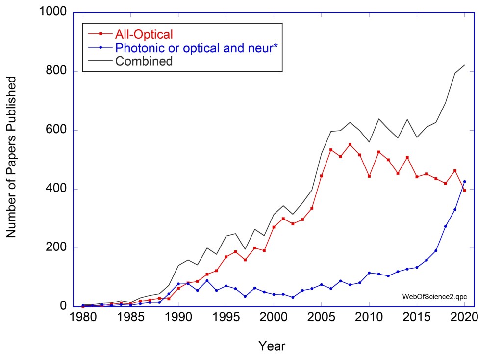
That said, it’s dangerous to ever say never, and research into all-optical computing and data processing is still going strong (See Fig. 1). It’s not the dream that was wrong, it was the time-scale that was wrong, just like fiber-to-the-home. Back in 2001, fiber-to-the-home was viewed as a pipe-dream by serious technology scouts. It took twenty years, but now that vision is coming true in urban settings. Back in 2001, all-optical computing seemed about 20 years away, but now it still looks 20 years out. Maybe this time the prediction is right. Recent advances in all-optical processing give some hope for it. Here are some of those advances.

Fig. 1 Number of papers published by year with the phrase in the title: “All-Optical” or “Photonic or Optical and Neur*” according to Web of Science search. The term “All-optical” saturated around 2005. Papers written around optical neural networks was low to 2015 but now is experiencing a strong surge. The sociology of title choices, and how favorite buzz words shift over time, can obscure underlying causes and trends, but overall there is current strong interest in all-optical systems.

The “What” and “Why” of All-Optical Processing

One of the great dreams of photonics is the use of light beams to perform optical logic in optical processors just as electronic currents perform electronic logic in transistors and integrated circuits.

Our information age, starting with the telegraph in the mid-1800’s, has been built upon electronics because the charge of the electron makes it a natural decision maker. Two charges attract or repel by Coulomb’s Law, exerting forces upon each other. Although we don’t think of currents acting in quite that way, the foundation of electronic logic remains electrical interactions.

But with these interactions also come constraints—constraining currents to be contained within wires, waiting for charging times that slow down decisions, managing electrical resistance and dissipation that generate heat (computer processing farms in some places today need to be cooled by glacier meltwater). Electronic computing is hardly a green technology.

Therefore, the advantages of optical logic are clear: broadcasting information without the need for expensive copper wires, little dissipation or heat, low latency (signals propagate at the speed of light). Furthermore, information on the internet is already in the optical domain, so why not keep it in the optical domain and have optical information packets making the decisions? All the routing and switching decisions about where optical information packets should go could be done by the optical packets themselves inside optical computers.

But there is a problem. Photons in free space don’t interact—they pass through each other unaffected. This is the opposite of what is needed for logic and decision making. The challenge of optical logic is then to find a way to get photons to interact.

Think of the scene in Star Wars: The New Hope when Obiwan Kenobi and Darth Vader battle to the death in a light saber duel—beams of light crashing against each other and repelling each other with equal and opposite forces. This is the photonic engineer’s dream! Light controlling light. But this cannot happen in free space. On the other hand, light beams can control other light beams inside nonlinear crystals where one light beam changes the optical properties of the crystal, hence changing how another light beam travels through it. These are nonlinear optical crystals.

Nonlinear Optics

Virtually all optical control designs, for any kind of optical logic or switch, require one light beam to affect the properties of another, and that requires an intervening medium that has nonlinear optical properties. The physics of nonlinear optics is actually simple: one light beam changes the electronic structure of a material which affects the propagation of another (or even the same) beam. The key parameter is the nonlinear coefficient that determines how intense the control beam needs to be to produce a significant modulation of the other beam. This is where the challenge is. Most materials have very small nonlinear coefficients, and the intensity of the control beam usually must be very high.

Therefore, to create low-power all-optical logic gates and switches there are four main design principles: 1) increase the nonlinear susceptibility by engineering the material, 2) increase the interaction length between the two beams, 3) concentrate light into small volumes, and 4) introduce feedback to boost the internal light intensities. Let’s take these points one at a time.

Nonlinear susceptibility: The key to getting stronger interaction of light with light is in the ease with which a control beam of light can distort the crystal so that the optical conditions change for a signal beam. This is called the nonlinear susceptibility . When working with “conventional” crystals like semiconductors (e.g. CdZnSe) or rare-Earths (e.g. LiNbO₃), there is only so much engineering that is possible to try to tweak the nonlinear susceptibilities. However, artificially engineered materials can offer significant increases in nonlinear susceptibilities, these include plasmonic materials, metamaterials, organic semiconductors, photonic crystals. An increasingly important class of nonlinear optical devices are semiconductor optical amplifiers (SOA).

Interaction length: The interaction strength between two light waves is a product of the nonlinear polarization and the length over which the waves interact. Interaction lengths can be made relatively long in waveguides but can be made orders of magnitude longer in fibers. Therefore, nonlinear effects in fiber optics are a promising avenue for achieving optical logic.

Intensity Concentration: Nonlinear polarization is the product of the nonlinear susceptibility with the field amplitude of the waves. Therefore, focusing light down to small cross sections produces high power, as in the core of a fiber optic, again showing advantages of fibers for optical logic implementations.

Feedback: Feedback, as in a standing-wave cavity, increases the intensity as well as the effective interaction length by folding the light wave continually back on itself. Both of these effects boost the nonlinear interaction, but then there is an additional benefit: interferometry. Cavities, like a Fabry-Perot, are interferometers in which a slight change in the round-trip phase can produce large changes in output light intensity. This is an optical analog to a transistor in which a small control current acts as a gate for an exponential signal current. The feedback in the cavity of a semiconductor optical amplifier (SOA), with high internal intensities and long effective interaction lengths and an active medium with strong nonlinearity make these elements attractive for optical logic gates. Similarly, integrated ring resonators have the advantage of interferometric control for light switching. Many current optical switches and logic gates are based on SOAs and integrated ring resonators.

All-Optical Regeneration

The vision of the all-optical internet, where the logic operations that direct information to different locations is all performed by optical logic without ever converting into the electrical domain, is facing a barrier that is as challenging to overcome today as it was back in 2001: all-optical regeneration. All-optical regeneration has been and remains the Achilles Heal of the all-optical internet.

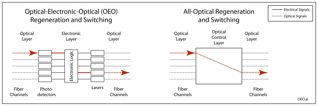
Signal regeneration is currently performed through OEO conversion: Optical-to-Electronic-to-Optical. In OEO conversion, a distorted signal (distortion is caused by attenuation and dispersion and noise as signals travel down fiber optics) is received by a photodetector, is interpreted as ones and zeros that drive laser light sources that launch the optical pulses down the next stretch of fiber. The new pulses are virtually perfect, but they again degrade as they travel, until they are regenerated, and so on. The added advantage of the electrical layer is that the electronic signals can be used to drive conventional electronic logic for switching.

In all-optical regeneration, on the other hand, the optical pulses need to be reamplified, reshaped and retimed––known as 3R regeneration––all by sending the signal pulses through nonlinear amplifiers and mixers, which may include short stretches of highly nonlinear fiber (HNLF) or semiconductor optical amplifiers (SOA). There have been demonstrations of 2R all-optical regeneration (reamplifying and reshaping but not retiming) at lower data rates, but getting all 3Rs at the high data rates (40 Gb/s) in the next generation telecom systems remains elusive.

Nonetheless, there is an active academic literature that is pushing the envelope on optical logical devices and regenerators [1]. Many of the systems focus on SOA’s, HNLF’s and Interferometers. Numerical modeling of these kinds of devices is currently ahead of bench-top demonstrations, primarily because of the difficulty of fabrication and device lifetime. But the numerical models point to performance that would be competitive with OEO. If this OOO conversion (Optical-to-Optical-to-Optical) is scalable (can handle increasing bit rates and increasing numbers of channels), then the current data crunch that is facing the telecom trunk lines (see my previous Blog) may be a strong driver to implement such all-optical solutions.

It is important to keep in mind that legacy technology is not static but also continues to improve. As all-optical logic and switching and regeneration make progress, OEO conversion gets incrementally faster, creating a moving target. Therefore, we will need to wait another 20 years to see whether OEO is overtaken and replaced by all-optical.

*Fig. 3 Optical-Electronic-Optical regeneration and switching compared to all-optical control. The optical control is performed using SOA’s, interferometers and nonlinear fibers.*

Photonic Neural Networks

The most exciting area of optical logic today is in analog optical computing––specifically optical neural networks and photonic neuromorphic computing [2, 3]. A neural network is a highly-connected network of nodes and links in which information is distributed across the network in much the same way that information is distributed and processed in the brain. Neural networks can take several forms––from digital neural networks that are implemented with software on conventional digital computers, to analog neural networks implemented in specialized hardware, sometimes also called neuromorphic computing systems.

Optics and photonics are well suited to the analog form of neural network because of the superior ability of light to form free-space interconnects (links) among a high number of optical modes (nodes). This essential advantage of light for photonic neural networks was first demonstrated in the mid-1980’s using recurrent neural network architectures implemented in photorefractive (nonlinear optical) crystals (see Fig. 1 for a publication timeline). But this initial period of proof-of-principle was followed by a lag of about 2 decades due to a mismatch between driver applications (like high-speed logic on an all-optical internet) and the ability to configure the highly complex interconnects needed to perform the complex computations.

Fig. 4 Optical vector-matrix multiplication. An LED array is the input vector, focused by a lens onto the spatial light modulator that is the 2D matrix. The transmitted light is refocussed by the lens onto a photodiode array with is the output vector. Free-space propagation and multiplication is a key advantage to optical implementation of computing.

The rapid rise of deep machine learning over the past 5 years has removed this bottleneck, and there has subsequently been a major increase in optical implementations of neural networks. In particular, it is now possible to use conventional deep machine learning to design the interconnects of analog optical neural networks for fixed tasks such as image recognition [4]. At first look, this seems like a non-starter, because one might ask why not use the conventional trained deep network to do the recognition itself rather than using it to create a special-purpose optical recognition system. The answer lies primarily in the metrics of latency (speed) and energy cost.

In neural computing, approximately 90% of the time and energy go into matrix multiplication operations. Deep learning algorithms driving conventional digital computers need to do the multiplications at the sequential clock rate of the computer using nested loops. Optics, on the other had, is ideally suited to perform matrix multiplications in a fully parallel manner (see Fig. 4). In addition, a hardware implementation using optics operates literally at the speed of light. The latency is limited only by the time of flight through the optical system. If the optical train is 1 meter, then the time for the complete computation is only a few nanoseconds at almost no energy dissipation. Combining the natural parallelism of light with the speed has led to unprecedented computational rates. For instance, recent implementations of photonic neural networks have demonstrated over 10 Trillion operations per second (TOPS) [5].

It is important to keep in mind that although many of these photonic neural networks are characterized as all-optical, they are generally not reconfigurable, meaning that they are not adaptive to changing or evolving training sets or changing input information. Most adaptive systems use OEO conversion with electronically-addressed spatial light modulators (SLM) that are driven by digital logic. Another technology gaining recent traction is neuromorphic photonics in which neural processing is implemented on photonic integrated circuits (PICS) with OEO conversion. The integration of large numbers of light emitting sources on PICs is now routine, relieving the OEO bottleneck as electronics and photonics merge in silicon photonics.

Farther afield are all-optical systems that are adaptive through the use of optically-addressed spatial light modulators or nonlinear materials. In fact, these types of adaptive all-optical neural networks were among the first demonstrated in the late 1980’s. More recently, advanced adaptive optical materials, as well as fiber delay lines for a type of recurrent neural network known as reservoir computing, have been used to implement faster and more efficient optical nonlinearities needed for adaptive updates of neural weights. But there are still years to go before light is adaptively controlling light entirely in the optical domain at the speeds and with the flexibility needed for real-world applications like photonic packet switching in telecom fiber-optic routers.

In stark contrast to the status of classical all-optical computing, photonic quantum computing is on the cusp of revolutionizing the field of quantum information science. The recent demonstration from the Canadian company Xanadu of a programmable photonic quantum computer that operates at room temperature may be the harbinger of what is to come in the third generation Machines of Light: Quantum Optical Computers, which is the topic of my next blog.

By David D. Nolte, Nov. 28, 2021

Galileo Unbound

Blogs inspired by the book Galileo Unbound (Oxford, 2018)

Tag / Deep Learning