Examples of conformal maps with transform functions for field lines and potentials.

September 3, 2025September 20, 2025 by David D. Nolte

The Craft of Conformal Maps

Somewhere, within the craft of conformal maps, lie the answers to dark, difficult problems of physics.

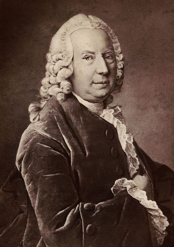
For instance, can you map out the electric field lines around one of Benjamin Franklin’s pointed lightning rods?

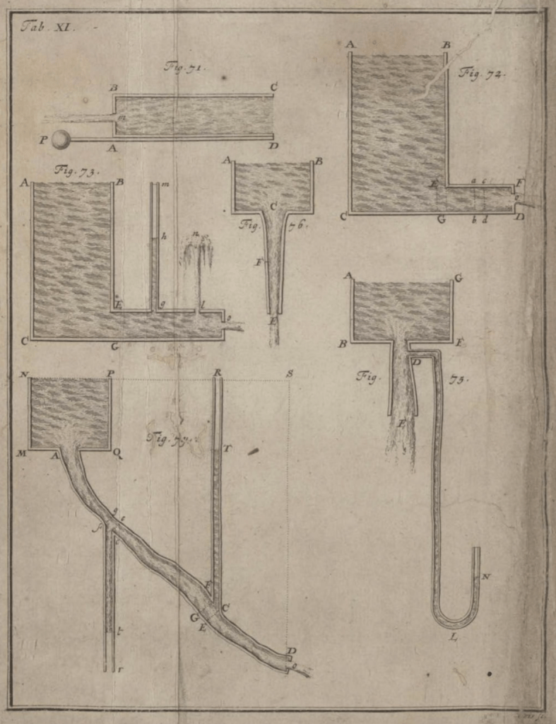
Can you calculate the fluid velocities in a channel making a sharp right angle?

Now take it up a notch in difficulty: Can you find the distribution of the sizes of magnetic domains within a flat magnet that is about to depolarize?

Or take it to the max: Can you find the vibration frequencies of the cosmic strings of string theory?

The answers to all these questions starts with simple physics solutions within simple boundaries—sometimes a problem so simple even a freshman physics student can solve it—and then mapping the solution, point by point, onto the geometry of the desired problem.

Once the right mapping function is found, you can solve some of the stickiest, ugliest, crankiest problems of physics like a pro.

The Earliest Conformal Maps

What is a conformal map? It is a transformation that takes one picture into another, keeping all local angles unchanged, no matter how distorted the overall transformation is.

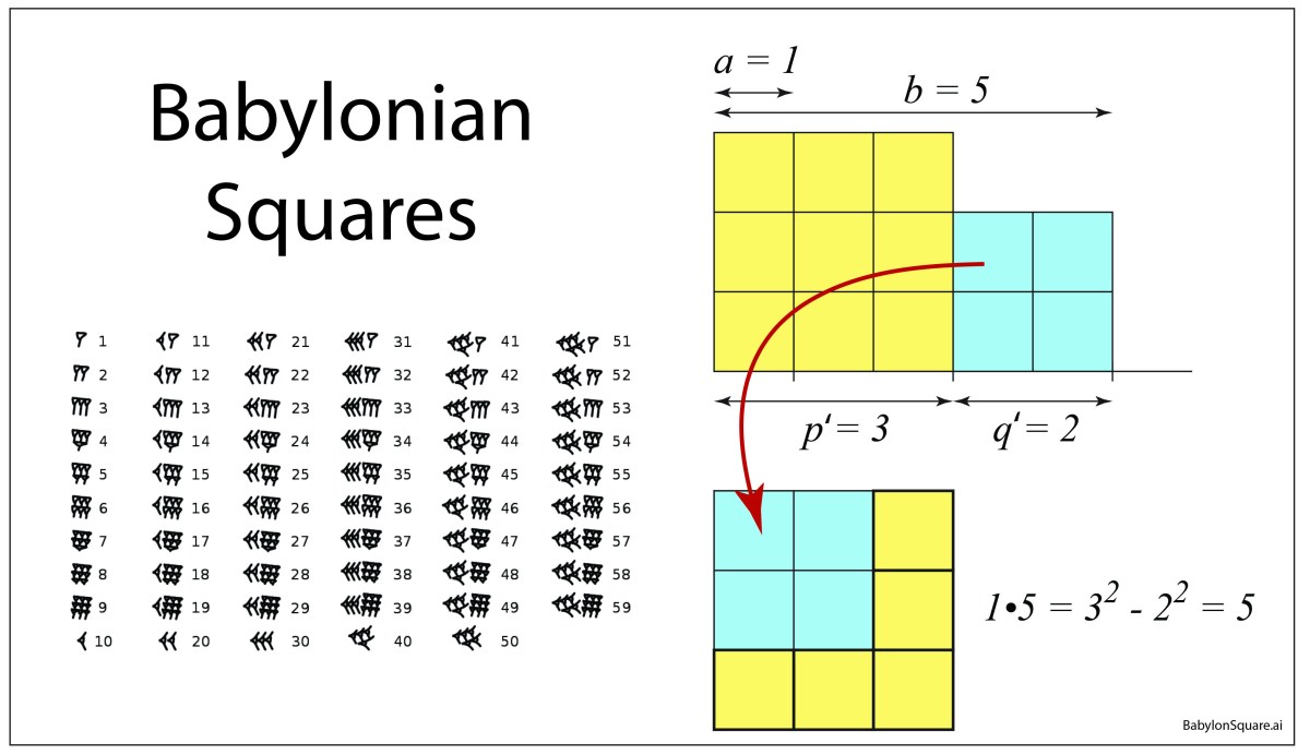
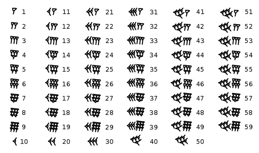
This property was understood by the very first mathematicians, wrangling their sexagesimal numbers by the waters of Babylon as they mapped the heavens onto charts to foretell the coming of the seasons.

Sterographic projection of the celestial sphere onto a plane — Fig. 1 Geometry of stereographic projection

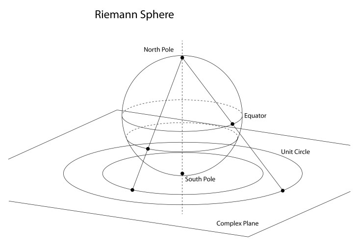
Hipparchus of Rhodes, around 150 BCE during the Hellenistic transition from Alexander to Caesar, was the first to describe the stereographic projection by which the locations of the stars were mapped on a plane by locating all the stars on the celestial sphere and tracing a line from the bottom of the sphere to the star and plotting where the line intersects the mid plane. Why this method should be conformal, preserving the angles, was probably beyond his mathematical powers, but he probably intuitively knew that it did.

Astrolabe map of the stars based on stereographic projection — Fig. 2 An astrolabe for the location of Brussels, Belgium, generated by a stereographic projection

Ptolemy of Alexandria around 150 CE, expanded on Hipparchus’ star charts and then introduced his own conical-like projection to map all the known world of his day. The Ptolemaic projection is almost conformal, but not quite. He was more interested in keeping areas faithful than angles.

Ptolemy's map of the world as reconstructed in the Renaissance. — Fig. 3 A Renaissance rendering of Ptolemy’s map of the known world in pseudo-conic projection.

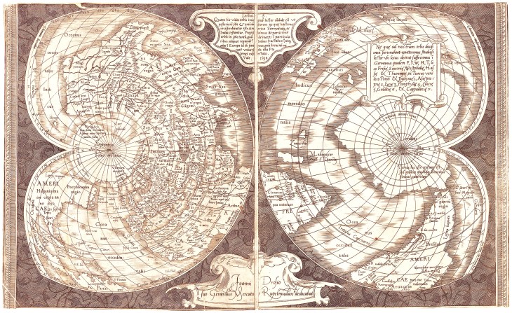
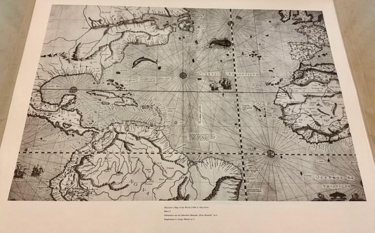
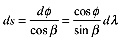
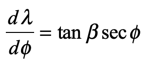
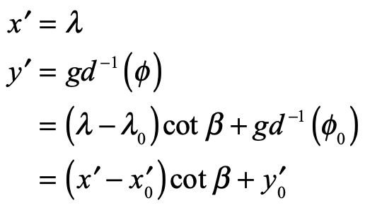
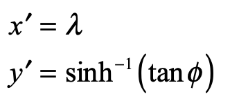
Mercator’s Rules of Rhumb

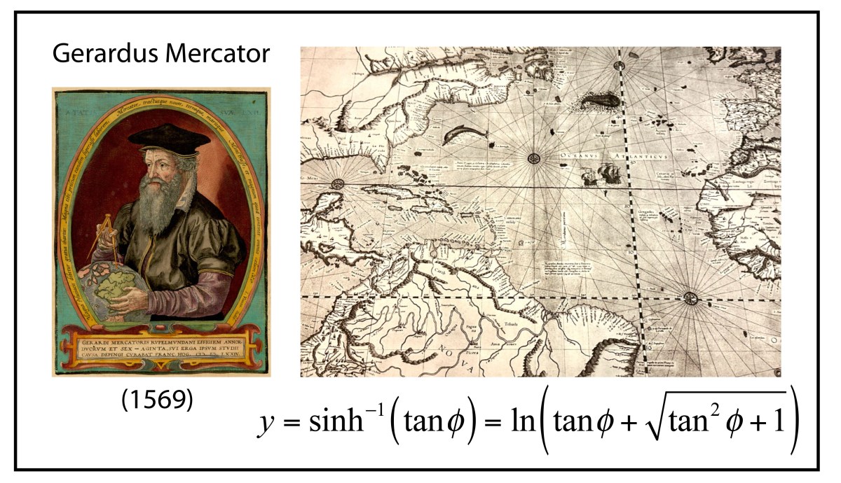
The first conformal mapping of the Earth’s surface onto the plane was constructed by Gerard Mercator in 1569. His goal, as a map maker, was to construct a map that traced out a ship’s course of constant magnetic bearing as a straight line, known as a rhumb line. This mapping property had important utility for navigators, especially on long voyages at sea beyond the sight of land, and was a hallmark of navigation maps of the Mediterranean, known as Portolan Charts. Rhumb lines were easy to draw on the small scales of the middle ocean, but on the scale of the Earth, no one knew how to do it.

Mercator's North Atlantic map — Fig. 4 Mercator’s North Atlantic with compass roses and rhumb lines. (Note the fictitious islands south of Iceland and the large arctic continent north of Greenland.)

Though Mercator’s life and career have been put under the biographer’s microscope numerous times, the exact moment when he realized how to make his map—the now-famous Mercator Projection—is not known. It is possible that he struck a compromise between a cylindrical point projection, that stretched the arctic regions, and a cylindrical line projection that compressed the arctic regions. He also was a maker of large globes on which rhumb lines (actually curves) could be measured and transferred to a flat map. Either way, he knew that he had invented something entirely new, and he promoted his map as an aid for the Age of Exploration. There is some evidence that Frobisher took Mercator’s map with him during his three famous arctic expeditions seeking the Northwest Passage.

Mercator projection of the Earth — Fig. 5 Modern Mercator conformal projection of the Earth.

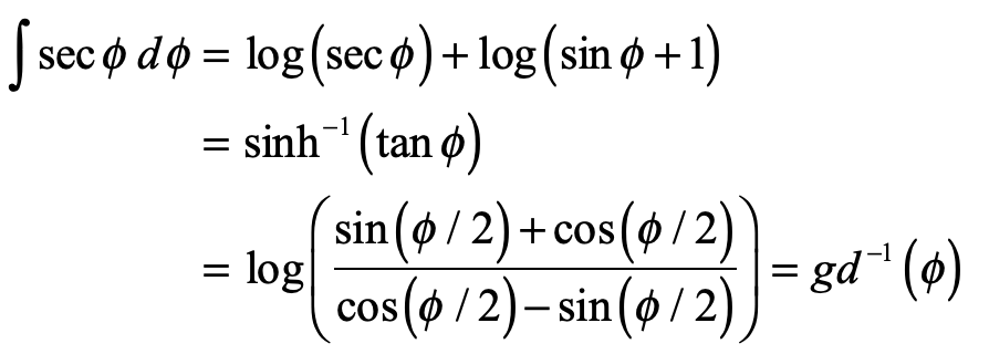
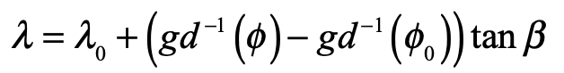
Mercator never explained nor described the mathematical function behind his projection. This was first discovered by the English mathematician Thomas Harriot in 1589, 20 years after Mercator published his map, as Harriot was helping Sir Walter Rayleigh with his New World projects. Like most of what Harriot did during his lifetime, he was years (sometimes decades) ahead of anyone else, but no one ever knew because he never published. His genius remained buried in his personal notes until they were uncovered in the late 1800’s long after others had claimed credit for things he did first.

The rhumb lines of Mercator’s map maintain constant angle relative to all lines of longitude and hence the Mercator projection is a conformal map. The mathematical proof of this fact was first given by James Gregory in 1668 (almost a century after Mercator’s feat) followed by a clearer proof by Isaac Barrow in 1670. It was 25 years later that Edmund Halley (of Halley’s Comet fame) proved that the stereographic projection was also conformal.

A hundred years passed after Halley before anyone again looked into the conformal properties of mapping—and then the field exploded.

The Rube in Frederick’s Berlin

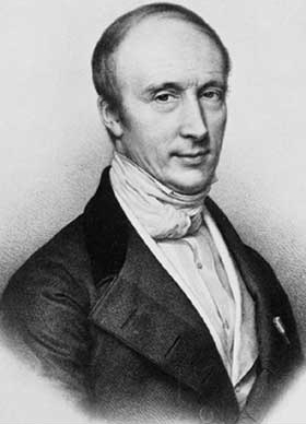
In 1761, the Swiss contingent of the Prussian Academy of Sciences nominated a little-known self-taught Swiss mathematician to the membership of the Academy. The process was pro forma, but everyone nominated was interviewed personally by Frederick the Great who had restructured the Academy years before from a backwater society to a leading scientific society in Europe. When Frederick met Johann Lambert, he thought it must be a practical joke. Lambert looked strange, dressed strangely, and his manners were even stranger. He was born poor, had never gone to school, and he looked it and he talked it.

Fig. 6 Portrait of Johann Heinrich Lambert

Frederick rejected the nomination.

But the Swiss contingent, led by Leonhard Euler himself, persisted, because they knew what Frederick did not—Lambert was a genius. He was an autodidact who had pulled himself up so thoroughly, that he had self-published some of the greatest works of philosophy and science of his generation. One of these was on the science of optics which established standards of luminance that we still use today. (In my own laboratory, my students and I routinely refer to Lambertian surfaces in our research on laser speckle. And we use the Lambert-Beer law of optical attenuation every day in our experiments.)

Frederick finally relented after a delay of two years, and admitted Lambert to his Academy, where Lambert went on a writing rampage, publishing a paper a month over the next ten years, like a dam letting loose.

One of Lambert’s many papers was on projection maps of the Earth. He not only picked up where Halley had left off a hundred years earlier, but he invented 7 new projections, three of which were conformal and four of which were equal area. Three of Lambert’s projections are in standard use today in cartography.

The Lambert conformal conic projection of the Earth — Fig. 7 The Lambert conformal conic projection centered on the 36th parallel.

Although Lambert worked at the time of Euler, Euler’s advances in complex-valued mathematics was still young and not well known, so Lambert worked his projections using conventional calculus. It would be another 100 years before the power of complex analysis was brought fully to bear on the problem of conformal mappings.

Riemann’s Sphere

It seems like the history of geometry can be divided into two periods: the time before Bernhard Riemann and the time after Bernhard Riemann.

Bernhard Riemann portrait — Fig. 8 Bernhard Riemann.

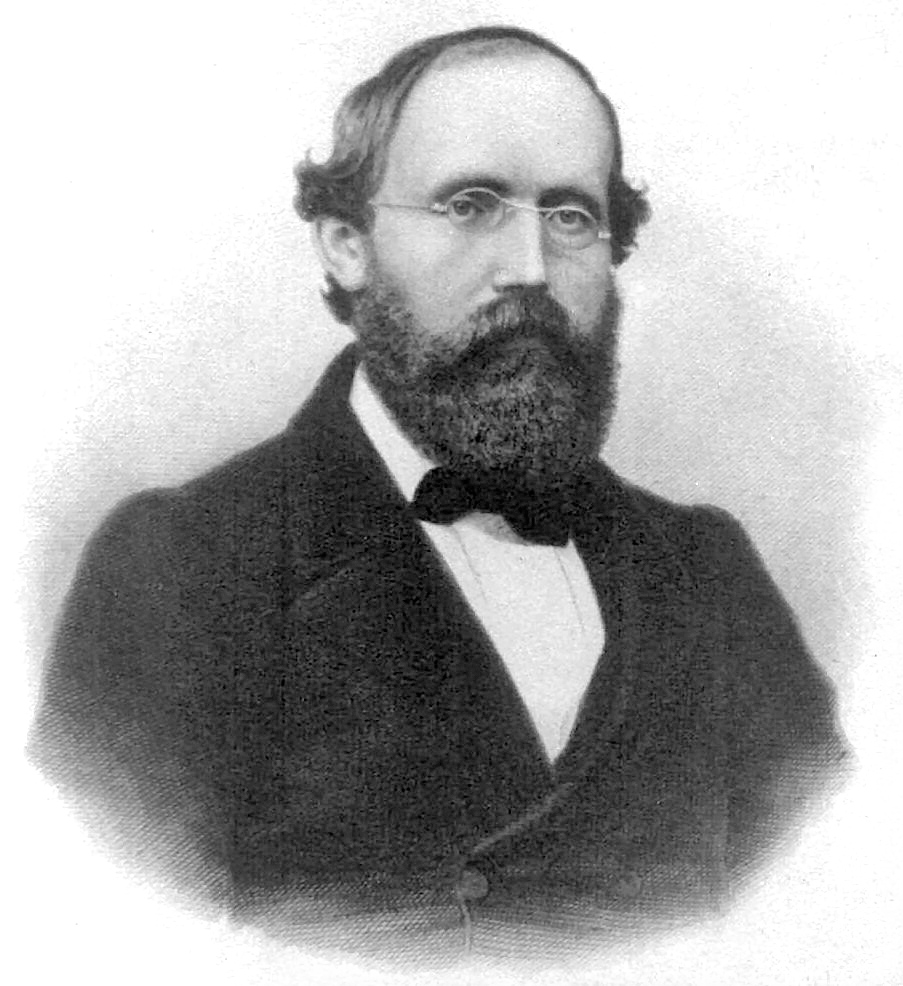
Bernhard Riemann was a gentle giant, a shy and unimposing figure with a Herculean mind. He transformed how everyone thought about geometry, both real and complex. His doctoral thesis was the most complete exposition to date on the power of complex analysis, and his Habilitation Lecture on the foundations of geometry shook those very foundations to their core.

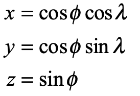
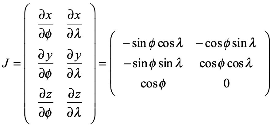
In the hands of Riemann, the stereographic projection became a complex transform of the simplest type

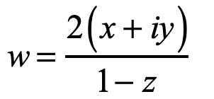
where x, y and z are the spherical coordinates of a point on the sphere.

Riemann sphere projection as a conformal map — Fig. 9 Conformal mapping of the surface of the Riemann sphere onto the complex plane.

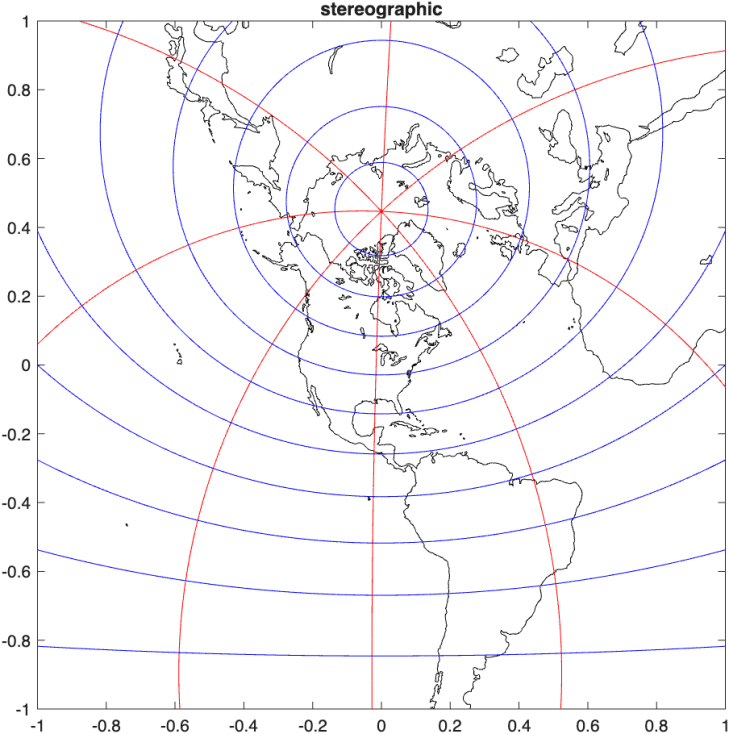
The projection in Fig. 9 is from the North Pole, which represents Antarctica faithfully but distorts the lands of the Northern Hemisphere. Any projection can be centered on a chosen point of the Earth by projecting from the opposite point, called the antipode. For instance, the stereographic projection centered on Chicago is shown in Fig. 10.

Stereographic projection centered on Chicago. — Fig. 10 Stereographic projection centered on Chicago, Illinois. Note the size of Greenland relative to its size in the Mercator projection of Fig. 5.

Building on the work of Euler and Cauchy, Riemann dove into conformal maps and emerged in 1851 with one of the most powerful theorems in complex analysis, known as the Riemann Mapping Theorem:

Any non-empty, simply connected open subset of the complex plane (which is not the entire plane itself) can be conformally mapped to the open unit disk.

An immediate consequence of this is that all non-empty, simply connected open subsets of the complex plane are equivalent, because any domain can be mapped onto the unit disk, and then the unit disk can be mapped to any domain.

The consequences of this are astounding: Solve a simple physics problem in a simple domain and then use the Riemann mapping theorem to transform it into the most complex, ugly, convoluted, twisted problem you can think of (as long as it is simply connected) and then you have the answer.

The reason that conformal maps (that are purely mathematical) allow the transformation of physics problems (that are “real”) is because physics is based on orthogonal sets of fields and potentials that govern how physical systems behave. In other words, the solution to the Laplacian operator on one domain can be transformed to a solution of the Laplacian operator on a different domain.

Powerful! Great! But how do you do it? Riemann’s theorem was an existence proof—not a solution manual. The mapping transformations still needed to be found.

Schwarz-Christoffel

On the heels of Bernard Riemann, who had altered the course of geometry, Hermann Schwarz at the University of Halle, Germany, and Elwin Bruno Christoffel at the Technical University in Zürich, Switzerland, took up Riemann’s mapping theorem to search for the actual mappings that would turn the theorem from “nice to know” to an actual formula.

Working independently, Christoffel in 1867 drew on his expertise in differential geometry while Schwarz in 1869 drew on his expertise in the calculus of variations, both with a solid background in geometry and complex analysis. They focused on conformal maps of polygons because general domains on the complex plane can be described with polygonal boundaries. The conformal map they sought would take simple portions of the complex plane and map them to the interior angle of a polygonal vertex. With sufficient constraints, the goal was to map all the vertexes and hence the entire domain.

The surprisingly simple result is known as the Schwarz-Christoffel equation

where a, b, c … are the positions of the vertices, and α, β, γ … are the interior angles of the vertices. The integral needs to be carried out on the complex plane, but it has closed-form solutions for many common cases.

This equation solves the problem of “how” that allows any physics solution on one domain to be mapped to another domain.

Conformal Maps

The list of possible conformal maps is literally limitless, yet there are a few that are so common that they deserve to be explored in some detail here.

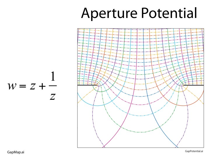
One conformal map is so “famous” it has the name of the Joukowski Map that takes the upper half plane and transforms it (through an open strip) onto the full complex plane. The field lines and potentials are shown in Fig. 11 as a simple transform of straight lines. To calculate these fields and potentials directly would require the solution of a partial differential equation (PDE) through numerical methods.

Field and potential lines near an aperture in conducting plates by a conformal map. — Fig. 11 Field lines and potentials around a gap in a charged conductor by the Joukowski conformal map.

Other common conformal maps are power-law transformations, taking the upper half plane into the full plane. Fig. 12 shows three of these, the first an inner half corner, the second the outer half corner, and the third transforming the upper half plane onto the full plane. All three of these show the field lines and the potentials near charged conducting plates.

Conformal maps from the half-plane to the full plane with field and potential lines. — Fig. 12 Maps from the half-plane to the full plane: a) Inner corner, b) outer corner, c) charged thin plate.

Conformal maps can also be “daisy-chained”. For instance, in Fig. 13, the unit circle is transformed into the upper half plane, providing the field lines and equipotentials of a point charge near a conducting plate. The fields are those of a point charge and its image charge, creating a dipole potential. This charge and its image are transformed again into the fields and potentials of a point charge near a conducting corner.

Compound conformal maps of the unit circle to the half-plane to the outside of a corner. — Fig. 13 Point charge fields and potentials near a conducting corner by a compound conformal map: a) Unit circle to the half-plane, b) Half-plane to the outside corder.

But we are not quite done with conformal maps. They have reappeared in recent years in exciting new areas of physics in the form of conformal field theory.

Conformal Field Theory

The importance being conformal extends far beyond solutions to Laplace’s equation. Physics is physics, regardless of how it comes about and how it is described, and transformations cannot change the physics. As an example, when a many-body system is at a critical point, then the description of the system is scale independent. In this case, changing scale is one type of transformation that keeps the physics the same. Conformal maps also keep the physics the same by preserving angles. Taking this idea into the quantum realm, a quantum field theory of a scale-invariant system can be conformally mapped onto other, more complex systems for which answers are not readily derived.

This is why conformal field theory (CFT) has become an important new field of physics with applications ranging as widely as quantum phase transitions and quantum strings.

Books by David Nolte at Oxford University Press — Read more in Books by David D. Nolte at Oxford University Press.

May 8, 2025September 3, 2025 by David D. Nolte

Magister Mercator Maps the World (1569)

Gerardus Mercator was born in no-man’s land, in Flanders’ fields, caught in the middle between the Protestant Reformation and the Holy Roman Empire. In his lifetime, armies washed back and forth over the countryside, sacking cities and obliterating the inhabitants. At age 32 he was imprisoned by the Inquisition for heresy, though he had committed none, and languished for months as the authorities searched for the slimmest evidence against him. They found none and he was released, though several of his fellow captives—elite academicians of their day—met their ends burned at the stake or beheaded or buried alive. It was not an easy time to be a scholar, with you and your work under persistent attack by political zealots.

Mercator received the degree of Magister, the degree in medieval universities that is equivalent to a Doctor of Philosophy … and then took what today we would call a “gap year” to “find himself” …

Yet in the midst of this turmoil and destruction, Mercator created marvels. Originally trained for the Church, he was bewitched by cartography at a time when the known world was expanding rapidly after the discoveries of the New World. Though the cognoscenti had known that the Earth was spherical since long before the Greeks, everyone saw it as flat, including cartographers, who in practice had to render it on flat maps. When the world was local, flat maps worked well. But as the world became global, new cartography methods were needed to capture the sphere, and Mercator entered the profession at just the moment when cartography was poised for a revolution.

Gerardus Mercator

The life of Gerardus Mercator (1512 – 1594) spanned nearly the full 16^th century. He was born 20 years after Colombus’ first voyage, and he died as Galileo began to study the law of fall, as Kepler began his study of planetary motion, and as Shakespeare began writing Romeo and Juliet. Mercator was born in the town of Rupelmonde, Flanders, outside of Antwerp in the southern part of the Netherlands ruled by Hapsburg Spain. His father was a poor shoemaker, but his uncle was an influential member of the clergy who paid for his nephew to attend a famous local school, in ‘s-Hertogenbosch, one where the humanist philosopher Erasmus (1466 – 1536) had attended several decades earlier.

Mercator entered the University of Leuven in 1530 in the humanities where his friends included Andreas Vesalius (the future famous anatomist) and Antoine Granvelle (who would become one of the most powerful Cardinals of the era). Mercator received the degree of Magister, the degree in medieval universities that is equivalent to a Doctor of Philosophy, in 1532, and then took what today we would call a “gap year” to “find himself” because he was having doubts about his faith and his future in the clergy. It was during his gap year that he was introduced to cartography by the Franciscan friar Franciscus Monachus (1490 – 1565) at the Mechelen monastery situated between Antwerp and Brussels.

Returning to the University of Leuven in 1534, he launched himself into the physical sciences of geography and mathematics, for which he had no training, but he quickly mastered them under the tutelage of the Dutch mapmaker Gemma Frisius (1508 – 1555) at the university. In 1537 Mercator completed his first map, a map of Palestine that received wide acclaim for its accuracy and artistry, and (more importantly) it sold well. He had found his vocation.

Early Cartography

Maps are among the oldest man-made textual artefacts, dating to nearly 7000 BCE, several millennia before the invention of writing itself. Knowing where things are, and where you are in relation to them, is probably the most important thing to remember in daily life. Texts are memory devices, and maps are the oldest texts.

The Alexandrian mathematician Claudius Ptolemy, around 150 CE, compiled a list of all the known world in his Geografia and drew up a map to accompany it. It survived through Arabic translation and became a fixture in early medieval Europe where it remained a record of virtually all that was known until Christopher Columbus ran into the Caribbean Islands in 1492 on his way to China. Maps needed to be redrawn.

A pseudo-conic projection of the Mediterranean attributed to Ptolemy. — Fig. 1. A 1482 reproduction of the map of Ptolemy from 150 BCE. The known world had not expanded much in 1000 years. There is no bottom to Africa (the voyage of Bartolomeu Dias around the Cape of Good Hope came 6 years later) and no New World (Columbus’s first voyage was 10 years off).

The first map to show the new world was printed in 1500 by the Castillan navigator Juan de la Cosa, who had sailed with Columbus three times. His map included the explorations of John Cabot to the northern coasts.

Portolan map by Juan de la Cosa. — **Fig. 2. Juan de la Cosa’s 1500 map showing the new world as a single landmass (dark green on the left). Europe, Africa and Asia are outlined in light lettering in the center and right.**

De la Cosa’s map was followed shortly by the world map of Martin Waldseemüller who named a small part of Brazil “America” in honor of Amerigo Vespucci who had just published an account of his adventures along the coasts of the new lands.

***Fig. 3. The Waldseemüller map of 1507 using “America” to name a part of current-day Brazil.***

Leonardo da Vinci went further and created an eight-octant map of the globe around 1514, calling the entire new landmass “America”, expanding on Waldseemüller’s use of the name beyond merely Brazil.

The gores of Leonardo's world. — Fig. 4. The eight-octant globe found in the Leonardo codex in England. The globe is likely not by Leonardo’s own hand, but by one of his followers created sometime after 1507. The detail has far less than on the Waldseemüller map, but it is notable because it calls all of the New World “America”.

In 1538, just a year after his success with his Palastine map, Mercator created a map of the world that showed for the first time the separation of the Americas into two continents, the North and the South, expanding the name “America” to its full modern extent.

Mercator's 1538 map of the world. — Fig. 5. Mercator’s 1538 World Map showing North America and South America as separate continents. This is a “double cordiform” projection, which is a modified conical projection onto an internal cone with the apex at the Poles and the base at the Equator. The cone is split along the international date line (long before that was created). The Arctic is shown as an ocean while the Antarctic is shown as a continent (long before either of these facts were known).

These maps by the early cartographers were not functional maps for navigation, but were large, sometimes many feet across, meant to be displayed to advantage on the spacious walls in the rooms of the rich and famous. On the other hand, since the late Middle Ages, there had been a long-standing tradition of map making among navigators whose lives depended on the utility and accuracy of their maps. These navigational charts were called Portolan Charts, meaning literally charts of ports or harbors. They carried sheaves of straight lines representing courses of constant magnetic bearing, meaning that the angle between the compass needle and the direction of the boat stayed constant. These are called rhumb lines, and they allowed ships to navigate between two known points beyond the sight of land. The importance of rhumb lines far surpassed the use of decorative maps. Mercator knew this, and for his next world map, he decided to give it rhumb lines that spanned the globe. The problem was how to do it.

Portolan chart of the central Mediterranean. — Fig. 6. A Portolan Chart of the Mediterranean with Italy and Greece at the center, outlined by light lettering by the names of ports and bays. The straight lines are rhumb lines for constant-bearing navigation.

A Conformal Projection

Around the time that Mercator was bursting upon the cartographic scene, a Portuguese mathematician, Pedro Nunes, was studying courses of constant bearing upon a spherical globe. These are mathematical paths on the sphere that were later called loxodromes, but over short distances, they corresponded to the rhumb line.

Thirty years later, Mercator had become a master cartographer, creating globes along with scientific instruments and maps. His globes were among the most precise instruments of their day, and he learned how to draw accurate loxodromes, following the work of Nunes. On a globe, these lines became “curly cues” as they approached a Pole of the sphere, circling around the Pole in ever tighter circles that defied mathematical description (until many years later when Thomas Harriot showed they were logarithmic spirals). Yet Mercator was a master draftsman, and he translated the curved loxodromes on the globe into straight lines on a world map. What he discovered was a projection in which all lines of Longitude and all lines of Meridian were straight lines, as were all courses of constant bearing. He completed his map in 1569, explicitly hawking its utility as a map that could be used on a global scale just as Portolan charts had been used in the Mediterranean.

Map of the North Atlantic by Gerard Mercator. — ***Fig. 7. A portion of Mercator’s 1569 World Map. The island just south of Thule (Iceland) is purely fictitious. Mercator has also filled in the Arctic Ocean with a new continent.***

A segment of Mercator's 1569 map of the world. — ***Fig. 8. The Atlantic Ocean on Mercator’s 1569 map. Rhumb lines run true at all latitudes.***

Mercator in 1569 was already established and famous and an old hand at making maps, yet even he was impressed by the surprising unity of his discovery. Today, the Mercator projection is called a conformal map, meaning that all angles among intersecting lines on the globe are conserved in the planar projection, explaining the linear longitudes, latitudes and rhumbs.

The Geometry of Gerhardus Mercator

Mercator’s new projection is a convenient exercise in differential geometry. Begin with the transformation from spherical coordinates to Cartesian coordinates

where λ is the longitude and φ is the latitude. The Jacobian matrix is

Taking the transpose, and viewing each row as a new vector

creates the basis vectors of the spherical surface

A unit vector with constant heading at angle β is expressed in the new basis vectors as

and the path length and arc length along a constant-bearing path are related as

Equating common coefficients of the basis vectors gives

which is solved to yield the ordinary differential equation

This is integrated as

which is a logarithmic spiral. The special function is called “the inverse Gundermannian”. The longitude λ as a function of the latitude φ is solved as

To generate a Mercator rhumb, we only need to go back to a new set of Cartesian coordinates on a flat map

It is interesting to compare the Mercator projection to a conical projection onto a cylinder touching the sphere at its equator where the Mercator projection is

while the conical projection onto the cylinder is

Clearly, the two projections are essentially the same around the Equator, but deviate exponentially approaching the Poles.

The Mercator projection has the conformal advantage, but it also has the disadvantage that landmasses at increasing latitude increase in size relative to their physical size on the glove. Therefore, Greenland looks as big as Africa on a Mercator projection, while it is in fact only about the size of Texas. The exaggerated sizes of countries in the upper latitudes (like the USA and Europe) relative to tropical countries near the equator has been viewed as creating an unfair psychological bias of first-world countries over third-world countries. For this reason, Mercator projections are virtually never used today, with other map projections that retain relative sizes being now the most common.

References

Crane, N. (2002), Mercator: The Man who Mapped the Planet, Weidenfeld & Nicolson, London.

Kythe, P. K. (2019), Handbook of Conformal Mappings and Applications, CRC Press.

Monmonier, M. S. (2004), Rhumb Lines and Map Wars: A Social History of the Mercator Projection, University of Chicago Press.

Snyder, J. P. (2002), Flattening the earth: Two thousand years of map projections, 5. ed ed., The University of Chicago Press, Chicago

Taylor, A. (2004), The World of Gerard Mercator: The Mapmaker Who Revolutionized Geography, Walker & Company, New York.

Read more in Books by David D. Nolte at Oxford University Press

October 22, 2024September 5, 2025 by David D. Nolte

Counting by the Waters of Babylon: The Secrets of the Babylonian 60-by-60 Multiplication System

Could you memorize a 60-by-60 multiplication table? It has 1830 distinct numbers to memorize.

The answer today is an emphatic “No”! Remember how long it took you to memorize the 12-by-12 table when you were a school child!

But 4000 years ago, the ancient Babylonians were doing it just fine—or at least “half” fine. This is how.

How to Tally

In the ancient land of Sumer, the centralization of the economy, and the need of the government to control it, made it necessary to keep records of who owned what and who gave what to whom. Scribes recorded transactions initially as tally marks pressed into soft clay around 5000 years ago, but one can only put so many marks on a clay tablet before it is full.

Therefore, two inventions were needed to save space and time. The first invention was a symbol that could stand in for a collection of tally marks. Given the ten fingers we have on our hands, it is no surprise that this aggregate symbol stood for 10 units—almost every culture has some aspect of a base-10 number system. With just two symbols repeated, numbers into the tens are easily depicted, as in Fig. 1.

*Figure 1. Babylonian cuneiform numbers use agglutination and place notation*

But by 4000 years ago, tallies were ranging into the millions, and a more efficient numerical notation was needed. Hence, the second invention.

Place-value notation—an idea more abstract than the first—was so abstract that other cultures who drew from Mesopotamian mathematics, such as the Greeks and Romans, failed to recognize its power and adopt it.

Today, we are so accustomed to place-value notation that it is hard to recognize how ingenious it is—how orders of magnitude are so easily encompassed in a few groups of symbols that keep track of thousands or millions at the same time as single units. Our own decimal place-value system is from Hindu-Arabic numerals, which seems natural enough to us, but the mathematics of Old Babylon from the time of Hammurabi (1792 – 1750 BCE) was sexagesimal, based on the number 60.

Our symbol for one hundred (100) using sexagesimal would be a pair of numbers (1,40) meaning 1×60+4×10.

Our symbol for 119 would be (1, 59) meaning 1×60 + 5×10 + 9.

Very large numbers are easily expressed. Our symbol for 13,179,661 (using eight symbols) would be expressed in the sexagesimal system using only 5 symbols as (1, 1, 1, 1, 1) for 1×60⁴+ 1×60³+ 1×60²+ 1×60 + 1.

There has been much speculation on why a base 60 numeral system makes any sense. The number does stand out because it has the largest number of divisors (1, 2, 3, 4, 5, 6, 10, 12, 15, 20, 30) of any smaller integer, and three of the divisors (2, 3, 5) are prime. Babylonian mathematical manipulation relied heavily on fractions, and the availability of so many divisors may have been the chief advantage of the system. The number the Babylonians used for the square root of 2 was (1; 24, 51, 10) = 1 + 24/60 + 51/60²+ 10/60³ = 1.41421296 which is accurate to almost seven decimal places. It has been pointed out [1] that this sexagesimal approximation for root-2 is what would be obtained if the Newton-Raphson method were used to find the root of the equation x²-2=0 starting from an initial guess of 3/2 = 1.5.

Squares, Products and Differences

One of the most important quantities in any civilization is the measurement of land areas. Land ownership is a measure of wealth and power and until recent times it was a requirement for authority or even citizenship. This remains true today when land possession and ownership are one the bricks in the foundation of social stability and status. The size of a McMansion is a status symbol, and the number of acres is a statement of wealth and power. Even renters are acutely aware of how many square feet they have in their apartment or house.

In ancient Sumer and Babylon, the possession of land was critically important, and it was necessary to measure land areas to track the accumulation or loss of ownership. Because the measurement of area requires the multiplication of numbers, it is no surprise that multiplication was one of the first mathematical developments.

Babylonian mathematics depended heavily on squares—literally square geometric figures—and the manipulation of squares formed their central algorithm for multiplication.

The algorithm begins by associating to any pair of number (a, b) a unique second pair (p’, q’) where p’ = (a+b)/2 is the semi-sum (known as the average), and q’ = (b-a)/2 is the semi-difference. The Babylonian mathematicians discovered that the product of the first pair is given by the difference in the squares of the second pair

as depicted in Fig. 2.

Figure 2. Old Babylonian mathematics. To a pair of numbers (a,b) is associated another pair (p’,q’): the average and the semi-difference. The product of the first pair of numbers is equal to the difference in the squares of the second pair (ab = p’² – q’²). A specific example is shown on the right.

This simple relation between products, and the differences of squares, provides a significant savings in time and effort when constructing products of two large numbers—as long as the two numbers have the same parity. That is the caveat! The semi-sum and semi-difference each must be an integer, which only happens when the two numbers share the same parity (evenness or oddness).

Therefore, while a multiplication table up to 60 by 60 would have 60•61/4 = 915 distinct numbers to memorize, which could not be memorized easily, all squares up to 60² gives just 60 numbers to memorize, which is fewer than our children need to learn today.

Therefore, with just 60 numbers, one could construct all 915 same-parity products of the 60 by 60 table using only sums and differences.

Try it yourself.

[1] pg. 60, R. L. Cooke, The History of Mathematics: A Brief Course. (New York, John Wiley & Sons, 2012)

Read more in Books by David Nolte at Oxford University Press

March 8, 2023September 3, 2025 by David D. Nolte

A Short History of Multiple Dimensions

Hyperspace by any other name would sound as sweet, conjuring to the mind’s eye images of hypercubes and tesseracts, manifolds and wormholes, Klein bottles and Calabi Yau quintics. Forget the dimension of time—that may be the most mysterious of all—but consider the extra spatial dimensions that challenge the mind and open the door to dreams of going beyond the bounds of today’s physics.

The geometry of n dimensions studies reality; no one doubts that. Bodies in hyperspace are subject to precise definition, just like bodies in ordinary space; and while we cannot draw pictures of them, we can imagine and study them.
(Poincare 1895)

Here is a short history of hyperspace. It begins with advances by Möbius and Liouville and Jacobi who never truly realized what they had invented, until Cayley and Grassmann and Riemann made it explicit. They opened Pandora’s box, and multiple dimensions burst upon the world never to be put back again, giving us today the manifolds of string theory and infinite-dimensional Hilbert spaces.

August Möbius (1827)

Although he is most famous for the single-surface strip that bears his name, one of the early contributions of August Möbius was the idea of barycentric coordinates [1] , for instance using three coordinates to express the locations of points in a two-dimensional simplex—the triangle. Barycentric coordinates are used routinely today in metallurgy to describe the alloy composition in ternary alloys.

August Möbius illustration — August Möbius (1790 – 1868). Image.

Möbius’ work was one of the first to hint that tuples of numbers could stand in for higher dimensional space, and they were an early example of homogeneous coordinates that could be used for higher-dimensional representations. However, he was too early to use any language of multidimensional geometry.

Carl Jacobi (1834)

Carl Jacobi was a master at manipulating multiple variables, leading to his development of the theory of matrices. In this context, he came to study (n-1)-fold integrals over multiple continuous-valued variables. From our modern viewpoint, he was evaluating surface integrals of hyperspheres.

Carl Gustav Jacob Jacobi photo — Carl Gustav Jacob Jacobi (1804 – 1851)

In 1834, Jacobi found explicit solutions to these integrals and published them in a paper with the imposing title “De binis quibuslibet functionibus homogeneis secundi ordinis per substitutiones lineares in alias binas transformandis, quae solis quadratis variabilium constant; una cum variis theorematis de transformatione et determinatione integralium multiplicium” [2]. The resulting (n-1)-fold integrals are

when the space dimension is even or odd, respectively. These are the surface areas of the manifolds called (n-1)-spheres in n-dimensional space. For instance, the 2-sphere is the ordinary surface 4πr² of a sphere on our 3D space.

Despite the fact that we recognize these as surface areas of hyperspheres, Jacobi used no geometric language in his paper. He was still too early, and mathematicians had not yet woken up to the analogy of extending spatial dimensions beyond 3D.

Joseph Liouville (1838)

Joseph Liouville’s name is attached to a theorem that lies at the core of mechanical systems—Liouville’s Theorem that proves that volumes in high-dimensional phase space are incompressible. Surprisingly, Liouville had no conception of high dimensional space, to say nothing of abstract phase space. The story of the convoluted path that led Liouville’s name to be attached to his theorem is told in Chapter 6, “The Tangled Tale of Phase Space”, in Galileo Unbound (Oxford University Press, 2018).

Joseph Liouville photo — Joseph Liouville (1809 – 1882)

Nonetheless, Liouville did publish a pure-mathematics paper in 1838 in Crelle’s Journal [3] that identified an invariant quantity that stayed constant during the differential change of multiple variables when certain criteria were satisfied. It was only later that Jacobi, as he was developing a new mechanical theory based on William R. Hamilton’s work, realized that the criteria needed for Liouville’s invariant quantity to hold were satisfied by conservative mechanical systems. Even then, neither Liouville nor Jacobi used the language of multidimensional geometry, but that was about to change in a quick succession of papers and books by three mathematicians who, unknown to each other, were all thinking along the same lines.

Liouville's theorem of 1838 — Facsimile of Liouville’s 1838 paper on invariants

Arthur Cayley (1843)

Arthur Cayley was the first to take the bold step to call the emerging geometry of multiple variables to be actual space. His seminal paper “Chapters in the Analytic Theory of n-Dimensions” was published in 1843 in the Philosophical Magazine [4]. Here, for the first time, Cayley recognized that the domain of multiple variables behaved identically to multidimensional space. He used little of the language of geometry in the paper, which was mostly analysis rather than geometry, but his bold declaration for spaces of n-dimensions opened the door to a changing mindset that would soon sweep through geometric reasoning.

Arthur Cayley painting — Arthur Cayley (1821 – 1895). Image

Hermann Grassmann (1844)

Grassmann’s life story, although not overly tragic, was beset by lifelong setbacks and frustrations. He was a mathematician literally 30 years ahead of his time, but because he was merely a high-school teacher, no-one took his ideas seriously.

Somehow, in nearly a complete vacuum, disconnected from the professional mathematicians of his day, he devised an entirely new type of algebra that allowed geometric objects to have orientation. These could be combined in numerous different ways obeying numerous different laws. The simplest elements were just numbers, but these could be extended to arbitrary complexity with arbitrary number of elements. He called his theory a theory of “Extension”, and he self-published a thick and difficult tome that contained all of his ideas [5]. He tried to enlist Möbius to help disseminate his ideas, but even Möbius could not recognize what Grassmann had achieved.

In fact, what Grassmann did achieve was vector algebra of arbitrarily high dimension. Perhaps more impressive for the time is that he actually recognized what he was dealing with. He did not know of Cayley’s work, but independently of Cayley he used geometric language for the first time describing geometric objects in high dimensional spaces. He said, “since this method of formation is theoretically applicable without restriction, I can define systems of arbitrarily high level by this method… geometry goes no further, but abstract science knows no limits.” [6]

Grassman was convinced that he had discovered something astonishing and new, which he had, but no one understood him. After years trying to get mathematicians to listen, he finally gave up, left mathematics behind, and actually achieved some fame within his lifetime in the field of linguistics. There is even a law of diachronic linguistics named after him. For the story of Grassmann’s struggles, see the blog on Grassmann and his Wedge Product .

Hermann Grassmann photo — Hermann Grassmann (1809 – 1877).

Julius Plücker (1846)

Projective geometry sounds like it ought to be a simple topic, like the projective property of perspective art as parallel lines draw together and touch at the vanishing point on the horizon of a painting. But it is far more complex than that, and it provided a separate gateway into the geometry of high dimensions.

A hint of its power comes from homogeneous coordinates of the plane. These are used to find where a point in three dimensions intersects a plane (like the plane of an artist’s canvas). Although the point on the plane is in two dimensions, it take three homogeneous coordinates to locate it. By extension, if a point is located in three dimensions, then it has four homogeneous coordinates, as if the three dimensional point were a projection onto 3D from a 4D space.

These ideas were pursued by Julius Plücker as he extended projective geometry from the work of earlier mathematicians such as Desargues and Möbius. For instance, the barycentric coordinates of Möbius are a form of homogeneous coordinates. What Plücker discovered is that space does not need to be defined by a dense set of points, but a dense set of lines can be used just as well. The set of lines is represented as a four-dimensional manifold. Plücker reported his findings in a book in 1846 [7] and expanded on the concepts of multidimensional spaces published in 1868 [8].

Jülius Plucker illustration — Julius Plücker (1801 – 1868).

Ludwig Schläfli (1851)

After Plücker, ideas of multidimensional analysis became more common, and Ludwig Schläfli (1814 – 1895), a professor at the University of Berne in Switzerland, was one of the first to fully explore analytic geometry in higher dimensions. He described multidimsnional points that were located on hyperplanes, and he calculated the angles between intersecting hyperplanes [9]. He also investigated high-dimensional polytopes, from which are derived our modern “Schläfli notation“. However, Schläffli used his own terminology for these objects, emphasizing analytic properties without using the ordinary language of high-dimensional geometry.

Polytopes by Schläfli — Some of the polytopes studied by Schläfli.

Bernhard Riemann (1854)

The person most responsible for the shift in the mindset that finally accepted the geometry of high-dimensional spaces was Bernhard Riemann. In 1854 at the university in Göttingen he presented his habilitation talk “Über die Hypothesen, welche der Geometrie zu Grunde liegen” (Over the hypotheses on which geometry is founded). A habilitation in Germany was an examination that qualified an academic to be able to advise their own students (somewhat like attaining tenure in US universities).

The habilitation candidate would suggest three topics, and it was usual for the first or second to be picked. Riemann’s three topics were: trigonometric properties of functions (he was the first to rigorously prove the convergence properties of Fourier series), aspects of electromagnetic theory, and a throw-away topic that he added at the last minute on the foundations of geometry (on which he had not actually done any serious work). Gauss was his faculty advisor and picked the third topic. Riemann had to develop the topic in a very short time period, starting from scratch. The effort exhausted him mentally and emotionally, and he had to withdraw temporarily from the university to regain his strength. After returning around Easter, he worked furiously for seven weeks to develop a first draft and then asked Gauss to set the examination date. Gauss initially thought to postpone to the Fall semester, but then at the last minute scheduled the talk for the next day. (For the story of Riemann and Gauss, see Chapter 4 “Geometry on my Mind” in the book Galileo Unbound (Oxford, 2018)).

Riemann gave his lecture on 10 June 1854, and it was a masterpiece. He stripped away all the old notions of space and dimensions and imbued geometry with a metric structure that was fundamentally attached to coordinate transformations. He also showed how any set of coordinates could describe space of any dimension, and he generalized ideas of space to include virtually any ordered set of measurables, whether it was of temperature or color or sound or anything else. Most importantly, his new system made explicit what those before him had alluded to: Jacobi, Grassmann, Plücker and Schläfli. Ideas of Riemannian geometry began to percolate through the mathematics world, expanding into common use after Richard Dedekind edited and published Riemann’s habilitation lecture in 1868 [10].

Bernhard Riemann photo — Bernhard Riemann (1826 – 1866). Image.

George Cantor and Dimension Theory (1878)

In discussions of multidimensional spaces, it is important to step back and ask what is dimension? This question is not as easy to answer as it may seem. In fact, in 1878, George Cantor proved that there is a one-to-one mapping of the plane to the line, making it seem that lines and planes are somehow the same. He was so astonished at his own results that he wrote in a letter to his friend Richard Dedekind “I see it, but I don’t believe it!”. A few decades later, Peano and Hilbert showed how to create area-filling curves so that a single continuous curve can approach any point in the plane arbitrarily closely, again casting shadows of doubt on the robustness of dimension. These questions of dimensionality would not be put to rest until the work by Karl Menger around 1926 when he provided a rigorous definition of topological dimension (see the Blog on the History of Fractals).

Peano curve compared to a Hilbert curve — Area-filling curves by Peano and Hilbert.

Hermann Minkowski and Spacetime (1908)

Most of the earlier work on multidimensional spaces were mathematical and geometric rather than physical. One of the first examples of physical hyperspace is the spacetime of Hermann Minkowski. Although Einstein and Poincaré had noted how space and time were coupled by the Lorentz equations, they did not take the bold step of recognizing space and time as parts of a single manifold. This step was taken in 1908 [11] by Hermann Minkowski who claimed

“Gentlemen! The views of space and time which I wish to lay before you … They are radical. Henceforth space by itself, and time by itself, are doomed to fade away into mere shadows, and only a kind of union of the two will preserve an independent reality.”Herman Minkowski (1908)

For the story of Einstein and Minkowski, see the Blog on Minkowski’s Spacetime: The Theory that Einstein Overlooked.

Hermann Minkowski's famous diagram of spacetime — Facsimile of Minkowski’s 1908 publication on spacetime.

Felix Hausdorff and Fractals (1918)

No story of multiple “integer” dimensions can be complete without mentioning the existence of “fractional” dimensions, also known as fractals. The individual who is most responsible for the concepts and mathematics of fractional dimensions was Felix Hausdorff. Before being compelled to commit suicide by being jewish in Nazi Germany, he was a leading light in the intellectual life of Leipzig, Germany. By day he was a brilliant mathematician, by night he was the author Paul Mongré writing poetry and plays.

In 1918, as the war was ending, he wrote a small book “Dimension and Outer Measure” that established ways to construct sets whose measured dimensions were fractions rather than integers [12]. Benoit Mandelbrot would later popularize these sets as “fractals” in the 1980’s. For the background on a history of fractals, see the Blog A Short History of Fractals.

Felix Hausdorff photo — Felix Hausdorff (1868 – 1942)

Illustration of Sierpinski Gasket with fractal dimension — Example of a fractal set with embedding dimension D_E = 2, topological dimension D_T = 1, and fractal dimension D_H = 1.585.

The Fifth Dimension of Theodore Kaluza (1921) and Oskar Klein (1926)

The first theoretical steps to develop a theory of a physical hyperspace (in contrast to merely a geometric hyperspace) were taken by Theodore Kaluza at the University of Königsberg in Prussia. He added an additional spatial dimension to Minkowski spacetime as an attempt to unify the forces of gravity with the forces of electromagnetism. Kaluza’s paper was communicated to the journal of the Prussian Academy of Science in 1921 through Einstein who saw the unification principles as a parallel of some of his own attempts [13]. However, Kaluza’s theory was fully classical and did not include the new quantum theory that was developing at that time in the hands of Heisenberg, Bohr and Born.

Oskar Klein was a Swedish physicist who was in the “second wave” of quantum physicists having studied under Bohr. Unaware of Kaluza’s work, Klein developed a quantum theory of a five-dimensional spacetime [14]. For the theory to be self-consistent, it was necessary to roll up the extra dimension into a tight cylinder. This is like a strand a spaghetti—looking at it from far away it looks like a one-dimensional string, but an ant crawling on the spaghetti can move in two dimensions—along the long direction, or looping around it in the short direction called a compact dimension. Klein’s theory was an early attempt at what would later be called string theory. For the historical background on Kaluza and Klein, see the Blog on Oskar Klein.

Klein-gordon equation compared to the Schrödinger and Dirac equations — The wave equations of Klein-Gordon, Schrödinger and Dirac.

John Campbell (1931): Hyperspace in Science Fiction

Art has a long history of shadowing the sciences, and the math and science of hyperspace was no exception. One of the first mentions of hyperspace in science fiction was in the story “Islands in Space’, by John Campbell [15], published in the Amazing Stories quarterly in 1931, where it was used as an extraordinary means of space travel.

In 1951, Isaac Asimov made travel through hyperspace the transportation network that connected the galaxy in his Foundation Trilogy [16].

Testez-vous : Isaac Asimov avait-il (entièrement) raison ? - Sciences et Avenir — Isaac Asimov (1920 – 1992)

John von Neumann and Hilbert Space (1932)

Quantum mechanics had developed rapidly through the 1920’s, but by the early 1930’s it was in need of an overhaul, having outstripped rigorous mathematical underpinnings. These underpinnings were provided by John von Neumann in his 1932 book on quantum theory [17]. This is the book that cemented the Copenhagen interpretation of quantum mechanics, with projection measurements and wave function collapse, while also establishing the formalism of Hilbert space.

Hilbert space is an infinite dimensional vector space of orthogonal eigenfunctions into which any quantum wave function can be decomposed. The physicists of today work and sleep in Hilbert space as their natural environment, often losing sight of its infinite dimensions that don’t seem to bother anyone. Hilbert space is more than a mere geometrical space, but less than a full physical space (like five-dimensional spacetime). Few realize that what is so often ascribed to Hilbert was actually formalized by von Neumann, among his many other accomplishments like stored-program computers and game theory.

John von Neumann in front of an early vacuum tube computer — John von Neumann (1903 – 1957). Image Credits.

Einstein-Rosen Bridge (1935)

One of the strangest entities inhabiting the theory of spacetime is the Einstein-Rosen Bridge. It is space folded back on itself in a way that punches a short-cut through spacetime. Einstein, working with his collaborator Nathan Rosen at Princeton’s Institute for Advanced Study, published a paper in 1935 that attempted to solve two problems [18]. The first problem was the Schwarzschild singularity at a radius r = 2M/c² known as the Schwarzschild radius or the Event Horizon. Einstein had a distaste for such singularities in physical theory and viewed them as a problem. The second problem was how to apply the theory of general relativity (GR) to point masses like an electron. Again, the GR solution to an electron blows up at the location of the particle at r = 0.

Einstain-Rosen bridge illustration in 3D — Einstein-Rosen Bridge. Image.

To eliminate both problems, Einstein and Rosen (ER) began with the Schwarzschild metric in its usual form

where it is easy to see that it “blows up” when r = 2M/c² as well as at r = 0. ER realized that they could write a new form that bypasses the singularities using the simple coordinate substitution

to yield the “wormhole” metric

It is easy to see that as the new variable u goes from -inf to +inf that this expression never blows up. The reason is simple—it removes the 1/r singularity by replacing it with 1/(r + ε). Such tricks are used routinely today in computational physics to keep computer calculations from getting too large—avoiding the divide-by-zero problem. It is also known as a form of regularization in machine learning applications. But in the hands of Einstein, this simple “bypass” is not just math, it can provide a physical solution.

It is hard to imagine that an article published in the Physical Review, especially one written about a simple variable substitution, would appear on the front page of the New York Times, even appearing “above the fold”, but such was Einstein’s fame this is exactly the response when he and Rosen published their paper. The reason for the interest was because of the interpretation of the new equation—when visualized geometrically, it was like a funnel between two separated Minkowski spaces—in other words, what was named a “wormhole” by John Wheeler in 1957. Even back in 1935, there was some sense that this new property of space might allow untold possibilities, perhaps even a form of travel through such a short cut.

As it turns out, the ER wormhole is not stable—it collapses on itself in an incredibly short time so that not even photons can get through it in time. More recent work on wormholes have shown that it can be stabilized by negative energy density, but ordinary matter cannot have negative energy density. On the other hand, the Casimir effect might have a type of negative energy density, which raises some interesting questions about quantum mechanics and the ER bridge.

Edward Witten’s 10+1 Dimensions (1995)

A history of hyperspace would not be complete without a mention of string theory and Edward Witten’s unification of the variously different 10-dimensional string theories into 10- or 11-dimensional M-theory. At a string theory conference at USC in 1995 he pointed out that the 5 different string theories of the day were all related through dualities. This observation launched the second superstring revolution that continues today. In this theory, 6 extra spatial dimensions are wrapped up into complex manifolds such as the Calabi-Yau manifold.

Iconic Calabi-Yau six-dimensional manifold — Two-dimensional slice of a six-dimensional Calabi-Yau quintic manifold.

Prospects

There is definitely something wrong with our three-plus-one dimensions of spacetime. We claim that we have achieved the pinnacle of fundamental physics with what is called the Standard Model and the Higgs boson, but dark energy and dark matter loom as giant white elephants in the room. They are giant, gaping, embarrassing and currently unsolved. By some estimates, the fraction of the energy density of the universe comprised of ordinary matter is only 5%. The other 95% is in some form unknown to physics. How can physicists claim to know anything if 95% of everything is in some unknown form?

The answer, perhaps to be uncovered sometime in this century, may be the role of extra dimensions in physical phenomena—probably not in every-day phenomena, and maybe not even in high-energy particles—but in the grand expanse of the cosmos.

By David D. Nolte, Feb. 8, 2023

Bibliography:

M. Kaku, R. O’Keefe, Hyperspace: A scientific odyssey through parallel universes, time warps, and the tenth dimension. (Oxford University Press, New York, 1994).

A. N. Kolmogorov, A. P. Yushkevich, Mathematics of the 19th century: Geometry, analytic function theory. (Birkhäuser Verlag, Basel ; 1996).

References:

[1] F. Möbius, in Möbius, F. Gesammelte Werke,, D. M. Saendig, Ed. (oHG, Wiesbaden, Germany, 1967), vol. 1, pp. 36-49.

[2] Carl Jacobi, “De binis quibuslibet functionibus homogeneis secundi ordinis per substitutiones lineares in alias binas transformandis, quae solis quadratis variabilium constant; una cum variis theorematis de transformatione et determinatione integralium multiplicium” (1834)

[3] J. Liouville, Note sur la théorie de la variation des constantes arbitraires. Liouville Journal 3, 342-349 (1838).

[4] A. Cayley, Chapters in the analytical geometry of n dimensions. Collected Mathematical Papers 1, 317-326, 119-127 (1843).

[5] H. Grassmann, Die lineale Ausdehnungslehre. (Wiegand, Leipzig, 1844).

[6] H. Grassmann quoted in D. D. Nolte, Galileo Unbound (Oxford University Press, 2018) pg. 105

[7] J. Plücker, System der Geometrie des Raumes in Neuer Analytischer Behandlungsweise, Insbesondere de Flächen Sweiter Ordnung und Klasse Enthaltend. (Düsseldorf, 1846).

[8] J. Plücker, On a New Geometry of Space (1868).

[9] L. Schläfli, J. H. Graf, Theorie der vielfachen Kontinuität. Neue Denkschriften der Allgemeinen Schweizerischen Gesellschaft für die Gesammten Naturwissenschaften 38. ([s.n.], Zürich, 1901).

[10] B. Riemann, Über die Hypothesen, welche der Geometrie zu Grunde liegen, Habilitationsvortrag. Göttinger Abhandlung 13, (1854).

[11] Minkowski, H. (1909). “Raum und Zeit.” Jahresbericht der Deutschen Mathematikier-Vereinigung: 75-88.

[12] Hausdorff, F.(1919).“Dimension und ausseres Mass,”Mathematische Annalen, 79: 157–79.

[13] Kaluza, Theodor (1921). “Zum Unitätsproblem in der Physik”. Sitzungsber. Preuss. Akad. Wiss. Berlin. (Math. Phys.): 966–972

[14] Klein, O. (1926). “Quantentheorie und fünfdimensionale Relativitätstheorie“. Zeitschrift für Physik. 37 (12): 895

[15] John W. Campbell, Jr. “Islands of Space“, Amazing Stories Quarterly (1931)

[16] Isaac Asimov, Foundation (Gnome Press, 1951)

[17] J. von Neumann, Mathematical Foundations of Quantum Mechanics. (Princeton University Press, ed. 1996, 1932).

[18] A. Einstein and N. Rosen, “The Particle Problem in the General Theory of Relativity,” Phys. Rev. 48(73) (1935).

Interference (New from Oxford University Press: 2023)

Read about the history of light and interference.

Available at Amazon.

Available at Oxford U Press

Avaliable at Barnes & Nobles

December 17, 2022September 5, 2025 by David D. Nolte

Paul Dirac’s Delta Function

Physical reality is nothing but a bunch of spikes and pulses—or glitches. Take any smooth phenomenon, no matter how benign it might seem, and decompose it into an infinitely dense array of infinitesimally transient, infinitely high glitches. Then the sum of all glitches, weighted appropriately, becomes the phenomenon. This might be called the “glitch” function—but it is better known as Green’s function in honor of the ex-millwright George Green who taught himself mathematics at night to became one of England’s leading mathematicians of the age.

The δ function is thus merely a convenient notation … we perform operations on the abstract symbols, such as differentiation and integration …
PAM Dirac (1930)

The mathematics behind the “glitch” has a long history that began in the golden era of French analysis with the mathematicians Cauchy and Fourier, was employed by the electrical engineer Heaviside, and ultimately fell into the fertile hands of the quantum physicist, Paul Dirac, after whom it is named.

Augustin-Louis Cauchy (1815)

The French mathematician and physicist Augustin-Louis Cauchy (1789 – 1857) has lent his name to a wide array of theorems, proofs and laws that are still in use today. In mathematics, he was one of the first to establish “modern” functional analysis and especially complex analysis. In physics he established a rigorous foundation for elasticity theory (including the elastic properties of the so-called luminiferous ether).

In the early days of the 1800’s Cauchy was exploring how integrals could be used to define properties of functions. In modern terminology we would say that he was defining kernel integrals, where a function is integrated over a kernel to yield some property of the function.

In 1815 Cauchy read before the Academy of Paris a paper with the long title “Theory of wave propagation on a surface of a fluid of indefinite weight”. The paper was not published until more than ten years later in 1827 by which time it had expanded to 300 pages and contained numerous footnotes. The thirteenth such footnote was titled “On definite integrals and the principal values of indefinite integrals” and it contained one of the first examples of what would later become known as a generalized distribution. The integral is a function F(μ) integrated over a kernel

Cauchy lets the scale parameter α be “an infinitely small number”. The kernel is thus essentially zero for any values of μ “not too close to α”. Today, we would call the kernel given by

in the limit that α vanishes, “the delta function”.

Cauchy’s approach to the delta function is today one of the most commonly used descriptions of what a delta function is. It is not enough to simply say that a delta function is an infinitely narrow, infinitely high function whose integral is equal to unity. It helps to illustrate the behavior of the Cauchy function as α gets progressively smaller, as shown in Fig. 1.

Fig. 1 Cauchy function for decreasing scale factor α approaches a delta function in the limit.

In the limit as α approaches zero, the function grows progressively higher and progressively narrower, but the integral over the function remains unity.

Joseph Fourier (1822)

The delayed publication of Cauchy’s memoire kept it out of common knowledge, so it can be excused if Joseph Fourier (1768 – 1830) may not have known of it by the time he published his monumental work on heat in 1822. Perhaps this is why Fourier’s approach to the delta function was also different than Cauchy’s.

Fourier noted that an integral over a sinusoidal function, as the argument of the sinusoidal function went to infinity, became independent of the limits of integration. He showed

when ε << 1/p as p went to infinity. In modern notation, this would be the delta function defined through the “sinc” function

and Fourier noted that integrating this form over another function f(x) yielded the value of the function f(α) evaluated at α, rediscovering the results of Cauchy, but using a sinc(x) function in Fig. 2 instead of the Cauchy function of Fig. 1.

Fig. 2 Sinc function for increasing scale factor p approaches a delta function in the limit.

George Green’s Function (1829)

A history of the delta function cannot be complete without mention of George Green, one of the most remarkable British mathematicians of the 1800’s. He was a miller’s son who had only one year of education and spent most of his early life tending to his father’s mill. In his spare time, and to cut the tedium of his work, he read the most up-to-date work of the French mathematicians, reading the papers of Cauchy and Poisson and Fourier, whose work far surpassed the British work at that time. Unbelievably, he mastered the material and developed new material of his own, that he eventually self published. This is the mathematical work that introduced the potential function and introduced fundamental solutions to unit sources—what today would be called point charges or delta functions. These fundamental solutions are equivalent to the modern Green’s function, although they were developed rigorously much later by Courant and Hilbert and by Kirchhoff.

George Green’s flour mill in Sneinton, England.

The modern idea of a Green’s function is simply the system response to a unit impulse—like throwing a pebble into a pond to launch expanding ripples or striking a bell. To obtain the solutions for a general impulse, one integrates over the fundamental solutions weighted by the strength of the impulse. If the system response to a delta function impulse at x = a, that is, a delta function δ(x-a), is G(x-a), then the response of the system to a distributed force f(x) is given by

where G(x-a) is called the Green’s function.

Fig. Principle of Green’s function. The Green’s function is the system response to a delta-function impulse. The net system response is the integral over all the individual system responses summed over each of the impulses.

Oliver Heaviside (1893)

Oliver Heaviside (1850 – 1925) tended to follow his own path, independently of whatever the mathematicians were doing. Heaviside took particularly pragmatic approaches based on physical phenomena and how they might behave in an experiment. This is the context in which he introduced once again the delta function, unaware of the work of Cauchy or Fourier.

Heaviside was an engineer at heart who practiced his art by doing. He was not concerned with rigor, only with what works. This part of his personality may have been forged by his apprenticeship in telegraph technology helped by his uncle Charles Wheatstone (of the Wheatstone bridge). While still a young man, Heaviside tried to tackle Maxwell on his new treatise on electricity and magnetism, but he realized his mathematics were lacking, so he began a project of self education that took several years. The product of those years was his development of an idiosyncratic approach to electronics that may be best described as operator algebra. His algebra contained mis-behaved functions, such as the step function that was later named after him. It could also handle the derivative of the step function, which is yet another way of defining the delta function, though certainly not to the satisfaction of any rigorous mathematician—but it worked. The operator theory could even handle the derivative of the delta function.

The Heaviside function (step function) and its derivative the delta function.

Perhaps the most important influence by Heaviside was his connection of the delta function to Fourier integrals. He was one of the first to show that

which states that the Fourier transform of a delta function is a complex sinusoid, and the Fourier transform of a sinusoid is a delta function. Heaviside wrote several influential textbooks on his methods, and by the 1920’s these methods, including the Heaviside function and its derivative, had become standard parts of the engineer’s mathematical toolbox.

Given the work by Cauchy, Fourier, Green and Heaviside, what was left for Paul Dirac to do?

Paul Dirac (1930)

Paul Dirac (1902 – 1984) was given the moniker “The Strangest Man” by Niels Bohr during his visit to Copenhagen shortly after he had received his PhD. In part, this was because of Dirac’s internal intensity that could make him seem disconnected from those around him. When he was working on a problem in his head, it was not unusual for him to start walking, and by the time he he became aware of his surroundings again, he would have walked the length of the city of Copenhagen. And his solutions to problems were ingenious, breaking bold new ground where others, some of whom were geniuses themselves, were fumbling in the dark.

Among his many influential works—works that changed how physicists thought of and wrote about quantum systems—was his 1930 textbook on quantum mechanics. This was more than just a textbook, because it invented new methods by unifying the wave mechanics of Schrödinger with the matrix mechanics of Born and Heisenberg.

In particular, there had been a disconnect between bound electron states in a potential and free electron states scattering off of the potential. In the one case the states have a discrete spectrum, i.e. quantized, while in the other case the states have a continuous spectrum. There were standard quantum tools for decomposing discrete states by a projection onto eigenstates in Hilbert space, but an entirely different set of tools for handling the scattering states.

Yet Dirac saw a commonality between the two approaches. Specifically, eigenstate decomposition on the one hand used discrete sums of states, while scattering solutions on the other hand used integration over a continuum of states. In the first format, orthogonality was denoted by a Kronecker delta notation, but there was no equivalent in the continuum case—until Dirac introduced the delta function as a kernel in the integrand. In this way, the form of the equations with sums over states multiplied by Kronecker deltas took on the same form as integrals over states multiplied by the delta function.

Page 64 of Dirac’s 1930 edition of Quantum Mechanics.

In addition to introducing the delta function into the quantum formulas, Dirac also explored many of the properties and rules of the delta function. He was aware that the delta function was not a “proper” function, but by beginning with a simple integral property as a starting axiom, he could derive virtually all of the extended properties of the delta function, including properties of its derivatives.

Mathematicians, of course, were appalled and were quick to point out the insufficiency of the mathematical foundation for Dirac’s delta function, until the French mathematician Laurent Schwartz (1915 – 2002) developed the general theory of distributions in the 1940’s, which finally put the delta function in good standing.

Dirac’s introduction, development and use of the delta function was the first systematic definition of its properties. The earlier work by Cauchy, Fourier, Green and Heaviside had all touched upon the behavior of such “spiked” functions, but they had used it in passing. After Dirac, physicists embraced it as a powerful new tool in their toolbox, despite the lag in its formal acceptance by mathematicians, until the work of Schwartz redeemed it.

By David D. Nolte Feb. 17, 2022

Bibliography

V. Balakrishnan, “All about the Dirac Delta function(?)”, Resonance, Aug., pg. 48 (2003)

M. G. Katz. “Who Invented Dirac’s Delta Function?”, Semantic Scholar (2010).

J. Lützen, The prehistory of the theory of distributions. Studies in the history of mathematics and physical sciences ; 7 (Springer-Verlag, New York, 1982).

June 20, 2022February 9, 2023 by David D. Nolte

George Cantor meets Machine Learning: Deep Discrete Encoders

Machine learning is characterized, more than by any other aspect, by the high dimensionality of the data spaces it seeks to find patterns in. Hence, one of the principle functions of machine learning is to reduce the dimensionality of the data to lower dimensions—a process known as dimensionality reduction.

There are two driving reasons to reduce the dimensionality of data:

First, typical dimensionalities faced by machine learning problems can be in the hundreds or thousands. Trying to visualize such high dimensions may sound mind expanding, but it is really just saying that a data problem may have hundreds or thousands of different data entries for a single event. And many, or even most, of those entries may not be independent. While many others may be pure noise—or at least not relevant to the pattern. Deep learning dimensionality reduction seeks to find the dependences—many of them nonlinear and non-single-valued (non-invertible)—and to reject the noise channels.

Second, the geometry of high dimension is highly unintuitive. Many of the things we take for granted in our pitifully low dimension of 3 (or 4 if you include time) just don’t hold in high dimensions. For instance, in very high dimensions almost all random vectors in a hyperspace are orthogonal, and almost all random unit vectors in the hyperspace are equidistant. Even the topology of landscapes in high dimensions is unintuitive—there are far more mountain ridges than mountain peaks—with profound consequences for dynamical processes such as random walks (see my Blog on a Random Walk in 10 Dimensions). In fact, we owe our evolutionary existence to this effect! Therefore, deep dimensionality reduction is a way to bring complex data down to a dimensionality where our intuition can be applied to “explain” the data.

But what is a dimension? And can you find the “right” dimensionality when performing dimensionality reduction? Once again, our intuition struggles with these questions, as first discovered by a nineteenth-century German mathematician whose mind-expanding explorations of the essence of different types of infinity shattered the very concept of dimension.

George Cantor

Georg Cantor (1845 – 1918) was born in Russia, and the family moved to Germany while Cantor was still young. In 1863, he enrolled at the University of Berlin where he sat on lectures by Weierstrass and Kronecker. He received his doctorate in 1867 and his Habilitation in 1869, moving into a faculty position at the University of Halle and remaining there for the rest of his career. Cantor published a paper early in 1872 on the question of whether the representation of an arbitrary function by a Fourier series is unique. He had found that even though the series might converge to a function almost everywhere, there surprisingly could still be an infinite number of points where the convergence failed. Originally, Cantor was interested in the behavior of functions at these points, but his interest soon shifted to the properties of the points themselves, which became his life’s work as he developed set theory and transfinite mathematics.

In 1878, in a letter to his friend Richard Dedekind, Cantor showed that there was a one-to-one correspondence between the real numbers and the points in any n-dimensional space. He was so surprised by his own result that he wrote to Dedekind “I see it, but I don’t believe it.” Previously, the ideas of a dimension, moving in a succession from one (a line) to two (a plane) to three (a volume) had been absolute. However, with his newly-discovered mapping, the solid concepts of dimension and dimensionality began to dissolve. This was just the beginning of a long history of altered concepts of dimension (see my Blog on the History of Fractals).

Mapping Two Dimensions to One

Cantor devised a simple mapping that is at once obvious and subtle. To take a specific example of mapping a plane to a line, one can consider the two coordinate values (x,y) both with a closed domain on [0,1]. Each can be expressed as a decimal fraction given by

These two values can be mapped to a single value through a simple “ping-pong” between the decimal digits as

If x and y are irrational, then this presents a simple mapping of a pair of numbers (two-dimensional coordinates) to a single number. In this way, the special significance of two dimensions relative to one dimension is lost. In terms of set theory nomenclature, the cardinality of the two-dimensional R² is the same as for the one-dimensions R.

Nonetheless, intuition about dimension still has it merits, and a subtle aspect of this mapping is that it contains discontinuities. These discontinuities are countably infinite, but they do disrupt any smooth transformation from 2D to 1D, which is where the concepts of intrinsic dimension are hidden. The topological dimension of the plane is clearly equal to 2, and that of the line is clearly equal to 1, determined by the dimensionality D+1 of cuts that are required to separate the sets. The area is separated by a D = 1 line, while the line is separated by a D= 0 point.

Fig. 1 A mapping of a 2D plane to a 1D line. Every point in the plane has an associated point on the line (except for a countably infinite number of special points … see the next figure.)

While the discontinuities help preserve the notions of dimension, and they are countably infinite (with the cardinality of the rational numbers), they pertain merely to the representation of number by decimals. As an example, in decimal notation for a number a = 14159/10⁵, one has two equivalent representations

trailing either infinitely many 0’s or infinitely many 9’s. Despite the fact that these representations point to the same number, when it is used as one of the pairs in the bijection of Fig. 1, it produces two distinctly different numbers of t in R. Fortunately, there is a way to literally sweep this under the rug. Any time one retrieves a number that has repeating 0’s or 9’s, simply sweep it to the right it by dividing by a power of 10 to a region of trailing zeros for a different number, call it b, as in Fig. 2. The shifted version of a will not overlap with the number b, because b also ends in repeating 0’s or 9’s and so is swept farther to the right, and so on to infinity, so none of these numbers overlap, each is distinct, and the mapping becomes what is known as a bijection with one-to-one correspondence.

Fig. 3 The “measure-zero” fix. Numbers that have two equivalent representations can be shifted to the right to replace other numbers that are shifted further to the right, and so on to infinity. There is infinite room within the reals to accommodate the countably infinite number of repeating-decimal numbers.

Space-Filling Curves

When the peripatetic mathematician Guiseppe Peano learned of Cantor’s result for the mapping of 2D to 1D, he sought to demonstrate the correspondence geometrically, and he constructed a continuous curve that filled space, publishing the method in Sur une courbe, qui remplit toute une aire plane [1] in 1890. The construction of Peano’s curve proceeds by taking a square and dividing it into 9 equal sub squares. Lines connect the centers of each of the sub squares. Then each sub square is divided again into 9 sub squares whose centers are all connected by lines. At this stage, the original pattern, repeated 9 times, is connected together by 8 links, forming a single curve. This process is repeated infinitely many times, resulting in a curve that passes through every point of the original plane square. In this way, a line is made to fill a plane. Where Cantor had proven abstractly that the cardinality of the real numbers was the same as the points in n-dimensional space, Peano created a specific example.

This was followed quickly by another construction, invented by David Hilbert in 1891, that divided the square into four instead of nine, simplifying the construction, but also showing that such constructions were easily generated [2]. The space-filling curves of Peano and Hilbert have the extreme properties that a one-dimensional curve approaches every point in a two-dimensional space. These curves have topological dimensionality of 1D and a fractal dimensionality of 2D.

Fig. 3 Peano’s (1890) and Hilbert’s (1891) plane-filling curves. When the iterations are taken to infinity, the curves approach every point of two-dimensional space arbitrarily closely, giving them a dimension D = 2.

A One-Dimensional Deep Discrete Encoder for MNIST

When performing dimensionality reduction in deep learning it is tempting to think that there is an underlying geometry to the data—as if they reside on some submanifold of the original high-dimensional space. While this can be the case (for which dimensionality reduction is called deep metric learning) more often there is no such submanifold. For instance, when there is a highly conditional nature to the different data channels, in which some measurements are conditional on the values of other measurements, then there is no simple contiguous space that supports the data.

It is also tempting to think that a deep learning problem has some intrinsic number of degrees of freedom which should be matched by the selected latent dimensionality for the dimensionality reduction. For instance, if there are roughly five degrees of freedom buried within a complicated data set, then it is tempting to believe that the appropriate latent dimensionality also should be chosen to be five. But this also is missing the mark.

Take, for example, the famous MNIST data set of hand-written digits from 0 to 9. Each digit example is contained in a 28-by28 two-dimensional array that is typically flattened to a 784-element linear vector that locates that single digit example within a 784-dimensional space. The goal is to reduce the dimensionality down to a manageable number—but what should the resulting latent dimensionality be? How many degrees of freedom are involved in writing digits? Furthermore, given that there are ten classes of digits, should the chosen dimensionality of the latent space be related to the number of classes?

To illustrate that the dimensionality of the latent space has little to do with degrees of freedom or the number of classes, let’s build a simple discrete encoder that encodes the MNIST data set to the one-dimensional line—following Cantor.

The deep network of the encoder can have a simple structure that terminates with a single neuron that has a piece-wise linear output. The objective function (or loss function) measures the squared distances of the outputs of the single neuron, after transformation by the network, to the associated values 0 to 9. And that is it! Train the network by minimizing the loss function.

Fig. 5 A deep encoder that encodes discrete classes to a one-dimensional latent variable.

The results of the linear encoder are shown in Fig. 6 (the transverse directions are only for ease of visualization…the classification is along the long axis). The different dots are specific digits, and the colors are the digit value. There is a clear trend from 1 through 10, although with this linear encoder there is substantial overlap among the point clouds.

Fig. 6 Latent space for a one-dimensional (line) encoder. The transverse dimensions are only for visualization.

Despite appearances, this one-dimensional discrete line encoder is NOT a form of regression. There is no such thing as 1.5 as the average of a 1-digit and a 2-digit. And 5 is not the average of a 4-digit and a 6-digit. The digits are images that have no intrinsic numerical value. Therefore, this one-dimensional encoder is highly discontinuous, and intuitive ideas about intrinsic dimension for continuous data remain secure.

Summary

The purpose of this Blog (apart from introducing Cantor and his ideas on dimension theory) was to highlight a key question of dimensionality reduction in representation theory: What is the intrinsic dimensionality of a dataset? The answer, in the case of discrete classes, is that there is no intrinsic dimensionality. Having 1 degree of freedom or 10 degrees of freedom, i.e. latent dimensionalities of 1 or 10, is mostly irrelevant. In ideal cases, one is just as good as the other.

On the other hand, for real-world data with its inevitable variability and finite variance, there can be reasons to choose one latent dimensionality over another. In fact, the “best” choice of dimensionality is one less than the number of classes. For instance, in the case of MNIST with its 10 classes, that is a 9-dimensional latent space. The reason this is “best” has to do with the geometry of high-dimensional simplexes, which will be the topic of a future Blog.

By David D. Nolte, June 20, 2022

[1] G.Peano: Sur une courbe, qui remplit toute une aire plane. Mathematische Annalen 36 (1890), 157–160.

[2] D. Hilbert, “Uber die stetige Abbildung einer Linie auf ein Fllichenstilck,” Mathemutische Anna/en, vol. 38, pp. 459-460, (1891)

October 6, 2020October 8, 2020 by David D. Nolte

The Bountiful Bernoullis of Basel

The task of figuring out who’s who in the Bernoulli family is a hard nut to crack. The Bernoulli name populates a dozen different theorems or physical principles in the history of science and mathematics, but each one was contributed by any of four or five different Bernoullis of different generations—brothers, uncles, nephews and cousins. What makes the task even more difficult is that any given Bernoulli might be called by several different aliases, while many of them shared the same name across generations. To make things worse, they often worked and published on each other’s problems.

To attribute a theorem to a Bernoulli is not too different from attributing something to the famous mathematical consortium called Nicholas Bourbaki. It’s more like a team rather than an individual. But in the case of Bourbaki, the goal was selfless anonymity, while in the case of the Bernoullis it was sometimes the opposite—bald-faced competition and one-up-manship coupled with jealousy and resentment. Fortunately, the competition tended to breed more output than less, and the world benefited from the family feud.

The Bernoulli Family Tree

The Bernoullis are intimately linked with the beautiful city of Basel, Switzerland, situated on the Rhine River where it leaves Switzerland and forms the border between France and Germany . The family moved there from the Netherlands in the 1600’s to escape the Spanish occupation.

The first Bernoulli born in Basel was Nikolaus Bernoulli (1623 – 1708), and he had four sons: Jakob I, Nikolaus, Johann I and Hieronymous I. The “I”s in this list refer to the fact, or the problem, that many of the immediate descendants took their father’s or uncle’s name. The long-lived family heritage in the roles of mathematician and scientist began with these four brothers. Jakob Bernoulli (1654 – 1705) was the eldest, followed by Nikolaus Bernoulli (1662 – 1717), Johann Bernoulli (1667 – 1748) and then Hieronymous (1669 – 1760). In this first generation of Bernoullis, the great mathematicians were Jakob and Johann. More mathematical equations today are named after Jakob, but Johann stands out because of the longevity of his contributions, the volume and impact of his correspondence, the fame of his students, and the number of offspring who also took up mathematics. Johann was also the worst when it came to jealousy and spitefulness—against his brother Jakob, whom he envied, and specifically against his son Daniel, whom he feared would eclipse him.

Jakob Bernoulli (aka James or Jacques or Jacob)

Jakob Bernoulli (1654 – 1705) was the eldest of the first generation of brothers and also the first to establish himself as a university professor. He held the chair of mathematics at the university in Basel. While his interests ranged broadly, he is known for his correspondences with Leibniz as he and his brother Johann were among the first mathematicians to apply Lebiniz’ calculus to solving specific problems. The Bernoulli differential equation is named after him. It was one of the first general differential equations to be solved after the invention of the calculus. The Bernoulli inequality is one of the earliest attempts to find the Taylor expansion of exponentiation, which is also related to Bernoulli numbers, Bernoulli polynomials and the Bernoulli triangle. A special type of curve that looks like an ellipse with a twist in the middle is the lemniscate of Bernoulli.

Perhaps Jakob’s most famous work was his Ars Conjectandi (1713) on probability theory. Many mathematical theorems of probability named after a Bernoulli refer to this work, such as Bernoulli distribution, Bernoulli’s golden theorem (the law of large numbers), Bernoulli process and Bernoulli trial.

Fig. Bernoulli numbers in Jakob’s *Ars Conjectandi* (1713)

Johann Bernoulli (aka Jean or John)

Jakob was 13 years older than his brother Johann Bernoulli (1667 – 1748), and Jakob tutored Johann in mathematics who showed great promise. Unfortunately, Johann had that awkward combination of high self esteem with low self confidence, and he increasingly sought to show that he was better than his older brother. As both brothers began corresponding with Leibniz on the new calculus, they also began to compete with one another. Driven by his insecurity, Johann also began to steal ideas from his older brother and claim them for himself.

A classic example of this is the famous brachistrochrone problem that was posed by Johann in the Acta Eruditorum in 1696. Johann at this time was a professor of mathematics at Gronigen in the Netherlands. He challenged the mathematical world to find the path of least time for a mass to travel under gravity between two points. He had already found one solution himself and thought that no-one else would succeed. Yet when he heard his brother Jakob was responding to the challenge, he spied out his result and then claimed it as his own. Within the year and a half there were 4 additional solutions—all correct—using different approaches. One of the most famous responses was by Newton (who as usual did not give up his method) but who is reported to have solved the problem in a day. Others who contributed solutions were Gottfried Leibniz, Ehrenfried Walther von Tschirnhaus, and Guillaume de l’Hôpital in addition to Jakob.

The participation of de l’Hôpital in the challenge was a particular thorn in Johann’s side, because de l’Hôpital had years earlier paid Johann to tutor him in Leibniz’ new calculus at a time when l’Hôpital knew nothing of the topic. What is today known as l’Hôpital’s theorem on ratios of limits in fact was taught to l’Hôpital by Johann. Johann never forgave l’Hôpital for publicizing the result—but l’Hôpital had the discipline to write a textbook while Johann did not. To be fair, l’Hôpital did give Johann credit in the opening of his book, but that was not enough for Johann who continued to carry his resentment.

When Jakob died of tuberculosis in 1705, Johann campaigned to replace him in his position as professor of mathematics and succeeded. In that chair, Johann had many famous students (Euler foremost among them, but also Maupertuis and Clairaut). Part of Johann’s enduring fame stems from his many associations and extensive correspondences with many of the top mathematicians of the day. For instance, he had a regular correspondence with the mathematician Varignon, and it was in one of these letters that Johann proposed the principle of virtual velocities which became a key axiom for Joseph Lagrange’s later epic work on the foundations of mechanics (see Chapter 4 in Galileo Unbound).

Johann remained in his chair of mathematics at Basel for almost 40 years. This longevity, and the fame of his name, guaranteed that he taught some of the most talented mathematicians of the age, including his most famous student Leonhard Euler, who is held by some as one of the four greatest mathematicians of all time (the others were Archimedes, Newton and Gauss) [1].

Nikolaus I Bernoulli

Nikolaus I Bernoulli (1687 – 1759, son of Nikolaus) was the cousin of Daniel and nephew to both Jacob and Johann. He was a well-known mathematician in his time (he briefly held Galileo’s chair in Padua), though few specific discoveries are attributed to him directly. He is perhaps most famous today for posing the “St. Petersburg Paradox” of economic game theory. Ironically, he posed this paradox while his cousin Nikolaus II Bernoulli (brother of Daniel Bernoulli) was actually in St. Petersburg with Daniel.

The St. Petersburg paradox is a simple game of chance played with a fair coin where a player must buy in at a certain price in order to place $2 in a pot that doubles each time the coin lands heads, and pays out the pot at the first tail. The average pay-out of this game has infinite expectation, so it seems that anyone should want to buy in at any cost. But most people would be unlikely to buy in even for a modest $25. Why? And is this perception correct? The answer was only partially provided by Nikolaus. The definitive answer was given by his cousin Daniel Bernoulli.

Daniel Bernoulli

Daniel Bernoulli (1700 – 1782, son of Johann I) is my favorite Bernoulli. While most of the other Bernoullis were more mathematicians than scientists, Daniel Bernoulli was more physicist than mathematician. When we speak of “Bernoulli’s principle” today, the fundamental force that allows birds and airplanes to fly, we are referring to his work on hydrodynamics. He was one of the earliest originators of economic dynamics through his invention of the utility function and diminishing returns, and he was the first to clearly state the principle of superposition, which lies at the heart today of the physics of waves and quantum technology.

While in St. Petersburg, Daniel conceived of the solution to the St. Petersburg paradox (he is the one who actually named it). To explain why few people would pay high stakes to play the game, he devised a “utility function” that had “diminishing marginal utility” in which the willingness to play depended on ones wealth. Obviously a wealthy person would be willing to pay more than a poor person. Daniel stated

The determination of the value of an item must not be based on the price, but rather on the utility it yields…. There is no doubt that a gain of one thousand ducats is more significant to the pauper than to a rich man though both gain the same amount.

He created a log utility function that allowed one to calculate the highest stakes a person should be willing to take based on their wealth. Indeed, a millionaire may only wish to pay $20 per game to play, in part because the average payout over a few thousand games is only about $5 per game. It is only in the limit of an infinite number of games (and an infinite bank account by the casino) that the average payout diverges.

Johann II Bernoulli

Daniel’s brother Johann II (1710 – 1790) published in 1736 one of the most important texts on the theory of light during the time between Newton and Euler. Although the work looks woefully anachronistic today, it provided one of the first serious attempts at understanding the forces acting on light rays and describing them mathematically [5]. Euler based his new theory of light, published in 1746, on much of the work laid down by Johann II. Euler came very close to proposing a wave-like theory of light, complete with a connection between frequency of wave pulses and colors, that would have preempted Thomas Young by more than 50 years. Euler, Daniel and Johann II as well as Nicholas II were all contemporaries as students of Johann I in Basel.

More Relations

Over the years, there were many more Bernoullis who followed in the family tradition. Some of these include:

Johann II Bernoulli (1710–1790; also known as Jean), son of Johann, mathematician and physicist

Johann III Bernoulli (1744–1807; also known as Jean), son of Johann II, astronomer, geographer and mathematician

Jacob II Bernoulli (1759–1789; also known as Jacques), son of Johann II, physicist and mathematician

Johann Jakob Bernoulli (1831–1913), art historian and archaeologist; noted for his Römische Ikonographie (1882 onwards) on Roman Imperial portraits

Ludwig Bernoully (1873 – 1928), German architect in Frankfurt

Hans Bernoulli (1876–1959), architect and designer of the Bernoullihäuser in Zurich and Grenchen SO

Elisabeth Bernoulli (1873-1935), suffragette and campaigner against alcoholism.

Notable marriages to the Bernoulli family include the Curies (Pierre Curie was a direct descendant to Johann I) as well as the German author Hermann Hesse (married to a direct descendant of Johann I).

References

[1] Calinger, Ronald S.. Leonhard Euler : Mathematical Genius in the Enlightenment, Princeton University Press (2015).

[2] Euler L and Truesdell C. Leonhardi Euleri Opera Omnia. Series secunda: Opera mechanica et astronomica XI/2. The rational mechanics of flexible or elastic bodies 1638-1788. (Zürich: Orell Füssli, 1960).

[3] D Speiser, Daniel Bernoulli (1700-1782), Helvetica Physica Acta 55 (1982), 504-523.

[4] Leibniz GW. Briefwechsel zwischen Leibniz, Jacob Bernoulli, Johann Bernoulli und Nicolaus Bernoulli. (Hildesheim: Olms, 1971).

[5] Hakfoort C. Optics in the age of Euler : conceptions of the nature of light, 1700-1795. (Cambridge: Cambridge University Press, 1995).

August 3, 2020November 14, 2023 by David D. Nolte

Brook Taylor’s Infinite Series

When Leibniz claimed in 1704, in a published article in Acta Eruditorum, to have invented the differential calculus in 1684 prior to anyone else, the British mathematicians rushed to Newton’s defense. They knew Newton had developed his fluxions as early as 1666 and certainly no later than 1676. Thus ensued one of the most bitter and partisan priority disputes in the history of math and science that pitted the continental Leibnizians against the insular Newtonians. Although a (partisan) committee of the Royal Society investigated the case and found in favor of Newton, the affair had the effect of insulating British mathematics from Continental mathematics, creating an intellectual desert as the forefront of mathematical analysis shifted to France. Only when George Green filled his empty hours with the latest advances in French analysis, as he tended his father’s grist mill, did British mathematics wake up. Green self-published his epic work in 1828 that introduced what is today called Green’s Theorem.

Yet the period from 1700 to 1828 was not a complete void for British mathematics. A few points of light shone out in the darkness, Thomas Simpson, Collin Maclaurin, Abraham de Moivre, and Brook Taylor (1685 – 1731) who came from an English family that had been elevated to minor nobility by an act of Cromwell during the English Civil War.

Growing up in Bifrons House

View of Bifrons House from sometime in the late-1600’s showing the Jacobean mansion and the extensive south gardens.

When Brook Taylor was ten years old, his father bought Bifrons House [1], one of the great English country houses, located in the county of Kent just a mile south of Canterbury. English country houses were major cultural centers and sources of employment for 300 years from the seventeenth century through the early 20th century. While usually being the country homes of nobility of all levels, from Barons to Dukes, sometimes they were owned by wealthy families or by representatives in Parliament, which was the case for the Taylors. Bifrons House had been built around 1610 in the Jacobean architectural style that was popular during the reign of James I. The house had a stately front façade, with cupola-topped square towers, gable ends to the roof, porches of a renaissance form, and extensive manicured gardens on the south side. Bifrons House remained the seat of the Taylor family until 1824 when they moved to a larger house nearby and let Bifrons first to a Marquess and then in 1828 to Lady Byron (ex-wife of Lord Byron) and her daughter Ada Lovelace (the mathematician famous for her contributions to early computer science). The Taylor’s sold the house in 1830 to the first Marquess Conyngham.

Taylor’s life growing up in the rarified environment of Bifrons House must have been like scenes out of the popular BBC TV drama Downton Abbey. The house had a large staff of servants and large grounds at the edge of a large park near the town of Patrixbourne. Life as the heir to the estate would have been filled with social events and fine arts that included music and painting. Taylor developed a life-long love of music during his childhood, later collaborating with Isaac Newton on a scientific investigation of music (it was never published). He was also an amateur artist, and one of the first books he published after being elected to the Royal Society was on the mathematics of linear perspective, which contained some of the early results of projective geometry.

There is a beautiful family portrait in the National Portrait Gallery in London painted by John Closterman around 1696. The portrait is of the children of John Taylor about a year after he purchased Bifrons House. The painting is notable because Brook, the heir to the family fortunes, is being crowned with a wreath by his two older sisters (who would not inherit). Brook was only about 11 years old at the time and was already famous within his family for his ability with music and numbers.

Portrait of the children of John Taylor around 1696. Brook Taylor is the boy being crowned by his sisters on the left. (National Portrait Gallery)

Taylor never had to go to school, being completely tutored at home until he entered St. John’s College, Cambridge, in 1701. He took mathematics classes from Machin and Keill and graduated in 1709. The allowance from his father was sufficient to allow him to lead the life of a gentleman scholar, and he was elected a member of the Royal Society in 1712 and elected secretary of the Society just two years later. During the following years he was active as a rising mathematician until 1721 when he married a woman of a good family but of no wealth. The support of a house like Bifrons always took money, and the new wife’s lack of it was enough for Taylor’s father to throw the new couple out. Unfortunately, his wife died in childbirth along with the child, so Taylor returned home in 1723. These family troubles ended his main years of productivity as a mathematician.

Methodus incrementorum directa et inversa

Under the eye of the Newtonian mathematician Keill at Cambridge, Taylor became a staunch supporter and user of Newton’s fluxions. Just after he was elected as a member of the Royal Society in 1712, he participated in an investigation of the priority for the invention of the calculus that pitted the British Newtonians against the Continental Leibnizians. The Royal Society found in favor of Newton (obviously) and raised the possibility that Leibniz learned of Newton’s ideas during a visit to England just a few years before Leibniz developed his own version of the differential calculus.

A re-evaluation of the priority dispute from today’s perspective attributes the calculus to both men. Newton clearly developed it first, but did not publish until much later. Leibniz published first and generated the excitement for the new method that dispersed its use widely. He also took an alternative route to the differential calculus that is demonstrably different than Newton’s. Did Leibniz benefit from possibly knowing Newton’s results (but not his methods)? Probably. But that is how science is supposed to work … building on the results of others while bringing new perspectives. Leibniz’ methods and his notations were superior to Newton’s, and the calculus we use today is closer to Leibniz’ version than to Newton’s.

Once Taylor was introduced to Newton’s fluxions, he latched on and helped push its development. The same year (1715) that he published a book on linear perspective for art, he also published a ground-breaking book on the use of the calculus to solve practical problems. This book, Methodus incrementorum directa et inversa, introduced several new ideas, including finite difference methods (which are used routinely today in numerical simulations of differential equations). It also considered possible solutions to the equation for a vibrating string for the first time.

The vibrating string is one of the simplest problem in “continuum mechanics”, but it posed a severe challenge to Newtonian physics of point particles. It was only much later that D’Alembert used Newton’s first law of action-reaction to eliminate internal forces to derive D’Alembert’s principle on the net force on an extended body. Yet Taylor used finite differences to treat the line mass of the string in a way that yielded a possible solution of a sine function. (To read about Taylor’s original contribution to the principle of superposition, see Chapter 2 of Interference.) Taylor was the first to propose that a sine function was the form of the string displacement during vibration. This idea would be taken up later by D’Alembert (who first derived the wave equation), and by Euler (who vehemently disagreed with D’Alembert’s solutions) and Daniel Bernoulli (who was the first to suggest that it is not just a single sine function, but a sum of sine functions, that described the string’s motion — the principle of superposition).

Of course, the most influential idea in Taylor’s 1715 book was his general use of an infinite series to describe a curve.

Taylor’s Series

Infinite series became a major new tool in the toolbox of analysis with the publication of John Wallis‘ Arithmetica Infinitorum published in 1656. Shortly afterwards many series were published such as Nikolaus Mercator‘s series (1668)

and James Gregory‘s series (1668)

And of course Isaac Newton’s generalized binomial theorem that he worked out famously during the plague years of 1665-1666

But these consisted mainly of special cases that had been worked out one by one. What was missing was a general method that could yield a series expression for any curve.

Taylor used concepts of finite differences as well as infinitesimals to derive his formula for expanding a function as a power series around any point. His derivation in Methodus incrementorum directa et inversa is not easily recognized today. Using difference tables, and ideas from Newton’s fluxions that viewed functions as curves traced out as a function of time, he arrived at the somewhat cryptic expression

where the “dots” are time derivatives, x stands for the ordinate (the function), v is a finite difference, and z is the abcissa moving with constant speed. If the abcissa moves with unit speed, then this becomes Taylor’s Series (in modern notation)

The term “Taylor’s series” was probably first used by L’Huillier in 1786, although Condorcet attributed the equation to both Taylor and d’Alembert in 1784. It was Lagrange in 1797 who immortalized Taylor by claiming that Taylor’s theorem was the foundation of analysis.

Example: sin(x)

Expand sin(x) around x = π

This is related to the expansion around x = 0 (also known as a Maclaurin series)

Example: arctan(x)

To get an feel for how to apply Taylor’s theorem to a function like arctan, begin with

and take the derivative of both sides

Rewrite this as

and substitute the expression for y

and integrate term by term to arrive at

This is James Gregory’s famous series. Although the math here is modern and only takes a few lines, it parallel’s Gregory’s approach. But Gregory had to invent aspects of calculus as he went along — his derivation covering many dense pages. In the priority dispute between Leibniz and Newton, Gregory is usually overlooked as an independent inventor of many aspects of the calculus. This is partly because Gregory acknowledged that Newton had invented it first, and he delayed publishing to give Newton priority.

Two-Dimensional Taylor’s Series

The ideas behind the Taylor’s series generalizes to any number of dimensions. For a scalar function of two variables it takes the form (out to second order)

where J is the Jacobian matrix (vector) and H is the Hessian matrix defined for the scalar function as

and

As a concrete example, consider the two-dimensional Gaussian function

The Jacobean and Hessian matrices are

which are the first- and second-order coefficients of the Taylor series.

References

[1] “A History of Bifrons House”, B. M. Thomas, Kent Archeological Society (2017)

BifronsHouse Download

[2] L. Feigenbaum, “TAYLOR,BROOK AND THE METHOD OF INCREMENTS,” Archive for History of Exact Sciences, vol. 34, no. 1-2, pp. 1-140, (1985)

[3] A. Malet, “GREGORIE, JAMES ON TANGENTS AND THE TAYLOR RULE FOR SERIES EXPANSIONS,” Archive for History of Exact Sciences, vol. 46, no. 2, pp. 97-137, (1993)

[4] E. Harier and G. Wanner, Analysis by its History (Springer, 1996)

Painting of Bifrons Park by Jan Wyck c. 1700

December 2, 2019February 27, 2023 by David D. Nolte

Hermann Grassmann’s Nimble Wedge Product

Hyperspace is neither a fiction nor an abstraction. Every interaction we have with our every-day world occurs in high-dimensional spaces of objects and coordinates and momenta. This dynamical hyperspace—also known as phase space—is as real as mathematics, and physics in phase space can be calculated and used to predict complex behavior. Although phase space can extend to thousands of dimensions, our minds are incapable of thinking even in four dimensions—we have no ability to visualize such things.

Grassmann was convinced that he had discovered a fundamentally new type of mathematics—he actually had.

Part of the trick of doing physics in high dimensions is having the right tools and symbols with which to work. For high-dimensional math and physics, one such indispensable tool is Hermann Grassmann’s wedge product. When I first saw the wedge product, probably in some graduate-level dynamics textbook, it struck me as a little cryptic. It is sort of like a vector product, but not, and it operated on things that had an intimidating name— “forms”. I kept trying to “understand” forms as if they were types of vectors. After all, under special circumstances, forms and wedges did produce some vector identities. It was only after I actually stepped back and asked myself how they were constructed that I realized that forms and wedge products were just a simple form of algebra, called exterior algebra. Exterior algebra is an especially useful form of algebra with simple rules. It goes far beyond vectors while harking back to a time before vectors even existed.

Hermann Grassmann: A Backwater Genius

We are so accustomed to working with oriented objects, like vectors that have a tip and tail, that it is hard to think of a time when that wouldn’t have been natural. Yet in the mid 1800’s, almost no one was thinking of orientations as a part of geometry, and it took real genius to conceive of oriented elements, how to manipulate them, and how to represent them graphically and mathematically. At a time when some of the greatest mathematicians lived—Weierstrass, Möbius, Cauchy, Gauss, Hamilton—it turned out to be a high school teacher from a backwater in Prussia who developed the theory for the first time.

Hermann Grassmann was the son of a high school teacher at the Gymnasium in Stettin, Prussia, (now Szczecin, Poland) and he inherited his father’s position, but at a lower level. Despite his lack of background and training, he had serious delusions of grandeur, aspiring to teach mathematics at the university in Berlin, even when he was only allowed to teach the younger high school students basic subjects. Nonetheless, Grassmann embarked on a program to educate himself, attending classes at Berlin in mathematics. As part of the requirements to be allowed to teach mathematics to the senior high-school students, he had to submit a thesis on an appropriate topic.

For years, he had been working on an idea that had originally come from his father about a mathematical theory that could manipulate abstract objects or concepts. He had taken this vague thought and had slowly developed it into a rigorous mathematical form with symbols and manipulations. His mind was one of those that could permute endlessly, and he defined and discovered dozens of different ways that objects could be defined and combined, and he wrote them all down in a tome of excessive size and complexity. When it was time to submit the thesis to the examiners, he had created a broad new system of algebra—at a time when no one recognized what a new algebra even meant, especially not his examiners, who could understand none of it. Fortunately, Grassmann had been corresponding with the famous German mathematician August Möbius over his ideas, and Möbius was encouraging and supportive, and the examiners accepted his thesis and allowed him to teach the upper class-men at his high school.

Encouraged by his success, Grassmann hoped that Möbius would help him climb even higher to teach in Berlin. Convinced that he had discovered a fundamentally new type of mathematics (he actually had), he decided to publish his thesis as a book under the title Die Lineale Ausdehnungslehre, ein neuer Zweig der Mathematik (The Theory of Linear Extension, a New Branch of Mathematics). He published it out of his own pocket. It is some measure of his delusion that he had thousands printed, but he sold almost none, and piles of the books were stored away to be used later as scrap paper. Möbius likewise distanced himself from Grassmann and his obsessive theories. Discouraged, Grassmann turned his back on mathematics, though he later achieved fame in the field of linguistics. (For more on Grassmann’s ideas and struggle for recognition, see Chapter 4 of Galileo Unbound).

Excerpt from Grassmann’s Ausdehnungslehre (Google Books).

The Odd Identity of Nicholas Bourbaki

If you look up the publication history of the famous French mathematician, Nicholas Bourbaki, you will be amazed to see a publication history that spans from 1935 to 2018 — over 85 years of publications! But if you look in the obituaries, you will see that he died in 1968. It’s pretty impressive to still be publishing 50 years after your death. JRR Tolkein has been doing that regularly, but few others spring to mind.

Actually, you have been duped! Nicholas is a fiction, constructed as a hoax by a group of French mathematicians who were simultaneously deadly serious about the need for a rigorous foundation on which to educate the new wave of mathematicians in the mid 20^th century. The group was formed during a mathematics meeting in 1924, organized by André Weil and joined by Henri Cartan (son of Eli Cartan), Claude Chevalley, Jean Coulomb, Jean Delsarte, Jean Dieudonné, Charles Ehresmann, René de Possel, and Szolem Mandelbrojt (uncle of Benoit Mandelbrot). They picked the last name of a French general, and Weil’s wife named him Nicholas. The group began publishing books under this pseudonym in 1935 and has continued until the present time. While their publications were entirely serious, the group from time to time had fun with mild hoaxes, such as posting his obituary on one occasion and a wedding announcement of his daughter on another.

The wedge product symbol took several years to mature. Eli Cartan’s book on differential forms published in 1945 used brackets to denote the product instead of the wedge. In Chevally’s book of 1946, he does not use the wedge, but uses a small square, and the book Chevalley wrote in 1951 “Introduction to the Theory of Algebraic Functions of One Variable” still uses a small square. But in 1954, Chevalley uses the wedge symbol in his book on Spinors. He refers to his own book of 1951 (which did not use the wedge) and also to the 1943 version of Bourbaki. The few existing copies of the 1943 Algebra by Bourbaki lie in obscure European libraries. The 1973 edition of the book does indeed use the wedge, although I have yet to get my hands on the original 1943 version. Therefore, the wedge symbol seems to have originated with Chevalley sometime between 1951 and 1954 and gained widespread use after that.

Exterior Algebra

Exterior algebra begins with the definition of an operation on elements. The elements, for example (u, v, w, x, y, z, etc.) are drawn from a vector space in its most abstract form as “tuples”, such that x = [x₁, x₂, x₃, …, x_n] in an n-dimensional space. On these elements there is an operation called the “wedge product”, the “exterior product”, or the “Grassmann product”. It is denoted, for example between two elements x and y, as x^y. It captures the sense of orientation through anti-commutativity, such that

As simple as this definition is, it sets up virtually all later manipulations of vectors and their combinations. For instance, we can immediately prove (try it yourself) that the wedge product of a vector element with itself equals zero

Once the elements of the vector space have been defined, it is possible to define “forms” on the vector space. For instance, a 1-form, also known as a vector, is any function

where a, b, c are scalar coefficients. The wedge product of two 1-forms

yields a 2-form, also known as a bivector. This specific example makes a direct connection to the cross product in 3-space as

where the unit vectors are mapped onto the 2-forms

Indeed, many of the vector identities of 3-space can be expressed in terms of exterior products, but these are just special cases, and the wedge product is more general. For instance, while the triple vector cross product is not associative, the wedge product is associative

which can give it an advantage when performing algebra on r-forms. Expressing the wedge product in terms of vector components

yields the immediate generalization to any number of dimensions (using the Einstein summation convention)

In this way, the wedge product expresses relationships in any number of dimensions.

A 3-form is constructed as the wedge product of 3 vectors

where the Levi-Civita permuation symbol has been introduced such that

Note that in 3-space there can be no 4-form, because one of the basis elements would be repeated, rendering the product zero. Therefore, the most general multilinear form for 3-space is

with 2³ = 8 elements: one scalar, three 1-forms, three 2-forms and one 3-form. In 4-space there are 2⁴ = 16 elements: one scalar, four 1-forms, six 2-forms, four 3-forms and one 4-form. So, the number of elements rises exponentially with the dimension of the space.

At this point, we have developed a rich multilinear structure, all based on the simple anti-commutativity of elements x^y = -y^x. This process is called by another name: a Clifford algebra, named after William Kingdon Clifford (1845-1879), second wrangler at Cambridge and close friend of Arthur Cayley. But the wedge product is not just algebra—there is also a straightforward geometric interpretation of wedge products that make them useful when extending theories of surfaces and volumes into higher dimensions.

Geometric Interpretation

In Euclidean space, a cross product is related to areas and volumes of paralellapipeds. Wedge products are more general than cross products and they generalize the idea of areas and volumes to higher dimension. As an illustration, an area 2-form is shown in Fig. 1 and a 3-form in Fig. 2.

Fig. 1 Area 2-form showing how the area of a parallelogram is related to the wedge product. The 2-form is an oriented area perpendicular to the unit vector.

Fig. 2 A volume 3-form in Euclidean space. The volume of the parallelogram is equal to the magnitude of the wedge product of the three vectors u, v, and w.

The wedge product is not limited to 3 dimensions nor to Euclidean spaces. This is the power and the beauty of Grassmann’s invention. It also generalizes naturally to differential geometry of manifolds producing what are called differential forms. When integrating in higher dimensions or on non-Euclidean manifolds, the most appropriate approach is to use wedge products and differential forms, which will be the topic of my next blog on the generalized Stokes’ theorem.

George Green’s Theorem

For a thirty-year old miller’s son with only one year of formal education, George Green had a strange hobby—he read papers in mathematics journals, mostly from France. This was his escape from a dreary life running a flour mill on the outskirts of Nottingham, England, in 1823. The tall wind mill owned by his father required 24-hour attention, with farmers depositing their grain at all hours and the mechanisms and sails needing constant upkeep. During his one year in school when he was eight years old he had become fascinated by maths, and he nurtured this interest after leaving school one year later, stealing away to the top floor of the mill to pore over books he scavenged, devouring and exhausting all that English mathematics had to offer. By the time he was thirty, his father’s business had become highly successful, providing George with enough wages to become a paying member of the private Nottingham Subscription Library with access to the Transactions of the Royal Society as well to foreign journals. This simple event changed his life and changed the larger world of mathematics.

French Analysis in England

George Green was born in Nottinghamshire, England. No record of his birth exists, but he was baptized in 1793, which may be assumed to be the year of his birth. His father was a baker in Nottingham, but the food riots of 1800 forced him to move outside of the city to the town of Sneinton, where he bought a house and built an industrial-scale windmill to grind flour for his business. He prospered enough to send his eight-year old son to Robert Goodacre’s Academy located on Upper Parliament Street in Nottingham. Green was exceptionally bright, and after one year in school he had absorbed most of what the Academy could teach him, including a smattering of Latin and Greek as well as French along with what simple math that was offered. Once he was nine, his schooling was over, and he took up the responsibility of helping his father run the mill, which he did faithfully, though unenthusiastically, for the next 20 years. As the milling business expanded, his father hired a mill manager that took part of the burden off George. The manager had a daughter Jane Smith, and in 1824 she had her first child with Green. Six more children were born to the couple over the following fifteen years, though they never married.

Without adopting any microscopic picture of how electric or magnetic fields are produced or how they are transmitted through space, Green could still derive rigorous properties that are independent of any details of the microscopic model.

During the 20 years after leaving Goodacre’s Academy, Green never gave up learning what he could, teaching himself to read French readily as well as mastering English mathematics. The 1700’s and early 1800’s had been a relatively stagnant period for English mathematics. After the priority dispute between Newton and Leibniz over the invention of the calculus, English mathematics had become isolated from continental advances. This was part snobbery, but also part handicap as the English school struggled with Newton’s awkward fluxions while the continental mathematicians worked with Leibniz’ more fruitful differential notation. One notable exception was Brook Taylor who developed the Taylor’s Series (and who grew up on the opposite end of the economic spectrum from Green, see my Blog on Taylor). However, the French mathematicians in the early 1800’s were especially productive, including such works as those by Lagrange, Laplace and Poisson.

One block away from where Green lived stood the Free Grammar School overseen by headmaster John Topolis. Topolis was a Cambridge graduate on a minor mission to update the teaching of mathematics in England, well aware that the advances on the continent were passing England by. For instance, Topolis translated Laplace’s mathematically advanced Méchaniqe Celéste from French into English. Topolis was also well aware of the work by the other French mathematicians and maintained an active scholarly output that eventually brought him back to Cambridge as Dean of Queen’s College in 1819 when Green was 26 years old. There is no record whether Topolis and Green knew each other, but their close proximity and common interests point to a natural acquaintance. One can speculate that Green may even have sought Topolis out, given his insatiable desire to learn more mathematics, and it is likely that Topolis would have introduced Green to the vibrant French school of mathematics.

By the time Green joined the Nottingham Subscription Library, he must already have been well trained in basic mathematics, and membership in the library allowed him to request loans of foreign journals (sort of like Interlibrary Loan today). With his library membership beginning in 1823, Green absorbed the latest advances in differential equations and must have begun forming a new viewpoint of the uses of mathematics in the physical sciences. This was around the same time that he was beginning his family with Jane as well as continuing to run his fathers mill, so his mathematical hobby was relegated to the dark hours of the night. Nonetheless, he made steady progress over the next five years as his ideas took rough shape and were refined until finally he took pen to paper, and this uneducated miller’s son began a masterpiece that would change the history of mathematics.

Essay on Mathematical Analysis of Electricity and Magnetism

By 1827 Green’s free-time hobby was about to bear fruit, and he took out a modest advertisement to announce its forthcoming publication. Because he was an unknown, and unknown to any of the local academics (Topolis had already gone back to Cambridge), he chose vanity publishing and published out of pocket. An Essay on the Application of Mathematical Analysis to the Theories of Electricity and Magnetism was printed in March of 1828, and there were 51 subscribers, mostly from among the members of the Nottingham Subscription Library who bought it at 7 shillings and 6 pence per copy, probably out of curiosity or sympathy rather than interest. Few, if any, could have recognized that Green’s little essay contained several revolutionary elements.

Fig. 1 Cover page of George Green’s Essay

The topic of the essay was not remarkable, treating mathematical problems of electricity and magnetism, which was in vogue at that time. As background, he had read works by Cavendish, Poisson, Arago, Laplace, Fourier, Cauchy and Thomas Young (probably Young’s Course of Lectures on Natural Philosopy and the Mechanical Arts (1807)). He paid close attention to Laplace’s treatment of celestial mechanics and gravitation which had obvious strong analogs to electrostatics and the Coulomb force because of the common inverse square dependence.

One radical contribution in Green’s essay was his introduction of the potential function—one of the first uses of the concept of a potential function in mathematical physics—and he gave it its modern name. Others had used similar constructions, such as Euler [1], D’Alembert [2], Laplace[3] and Poisson [4], but the use had been implicit rather than explicit. Green shifted the potential function to the forefront, as a central concept from which one could derive other phenomena. Another radical contribution from Green was his use of the divergence theorem. This has tremendous utility, because it relates a volume integral to a surface integral. It was one of the first examples of how measuring something over a closed surface could determine a property contained within the enclosed volume. Gauss’ law is the most common example of this, where measuring the electric flux through a closed surface determines the amount of enclosed charge. Lagrange in 1762 [5] and Gauss in 1813 [6] had used forms of the divergence theorem in the context of gravitation, but Green applied it to electrostatics where it has become known as Gauss’ law and is one of the four Maxwell equations. Yet another contribution was Green’s use of linear superposition to determine the potential of a continuous charge distribution, integrating the potential of a point charge over a continuous charge distribution. This was equivalent to defining what is today called a Green’s function, which is a common method to solve partial differential equations.

A subtle contribution of Green’s Essay, but no less influential, was his adoption of a mathematical approach to a physics problem based on the fundamental properties of the mathematical structure rather than on any underlying physical model. Without adopting any microscopic picture of how electric or magnetic fields are produced or how they are transmitted through space, he could still derive rigorous properties that are independent of any details of the microscopic model. For instance, the inverse square law of both electrostatics and gravitation is a fundamental property of the divergence theorem (a mathematical theorem) in three-dimensional space. There is no need to consider what space is composed of, such as the many differing models of the ether that were being proposed around that time. He would apply this same fundamental mathematical approach in his later career as a Cambridge mathematician to explain the laws of reflection and refraction of light.

George Green: Cambridge Mathematician

A year after the publication of the Essay, Green’s father died a wealthy man, his milling business having become very successful. Green inherited the family fortune, and he was finally able to leave the mill and begin devoting his energy to mathematics. Around the same time he began working on mathematical problems with the support of Sir Edward Bromhead. Bromhead was a Nottingham peer who had been one of the 51 subscribers to Green’s published Essay. As a graduate of Cambridge he was friends with Herschel, Babbage and Peacock, and he recognized the mathematical genius in this self-educated miller’s son. The two men spent two years working together on a pair of publications, after which Bromhead used his influence to open doors at Cambridge.

In 1832, at the age of 40, George Green enrolled as an undergraduate student in Gonville and Caius College at Cambridge. Despite his concerns over his lack of preparation, he won the first-year mathematics prize. In 1838 he graduated as fourth wrangler only two positions behind the future famous mathematician James Joseph Sylvester (1814 – 1897). Based on his work he was elected as a fellow of the Cambridge Philosophical Society in 1840. Green had finally become what he had dreamed of being for his entire life—a professional mathematician.

Green’s later papers continued the analytical dynamics trend he had established in his Essay by applying mathematical principles to the reflection and refraction of light. Cauchy had built microscopic models of the vibrating ether to explain and derive the Fresnel reflection and transmission coefficients, attempting to understand the structure of ether. But Green developed a mathematical theory that was independent of microscopic models of the ether. He believed that microscopic models could shift and change as newer models refined the details of older ones. If a theory depended on the microscopic interactions among the model constituents, then it too would need to change with the times. By developing a theory based on analytical dynamics, founded on fundamental principles such as minimization principles and geometry, then one could construct a theory that could stand the test of time, even as the microscopic understanding changed. This approach to mathematical physics was prescient, foreshadowing the geometrization of physics in the late 1800’s that would lead ultimately to Einsteins theory of General Relativity.

Green’s Theorem and Greens Function

Green died in 1841 at the age of 49, and his Essay was mostly forgotten. Ten years later a young William Thomson (later Lord Kelvin) was graduating from Cambridge and about to travel to Paris to meet with the leading mathematicians of the age. As he was preparing for the trip, he stumbled across a mention of Green’s Essay but could find no copy in the Cambridge archives. Fortunately, one of the professors had a copy that he lent Thomson. When Thomson showed the work to Liouville and Sturm it caused a sensation, and Thomson later had the Essay republished in Crelle’s journal, finally bringing the work and Green’s name into the mainstream.

In physics and mathematics it is common to name theorems or laws in honor of a leading figure, even if the they had little to do with the exact form of the theorem. This sometimes has the effect of obscuring the historical origins of the theorem. A classic example of this is the naming of Liouville’s theorem on the conservation of phase space volume after Liouville, who never knew of phase space, but who had published a small theorem in pure mathematics in 1838, unrelated to mechanics, that inspired Jacobi and later Boltzmann to derive the form of Liouville’s theorem that we use today. The same is true of Green’s Theorem and Green’s Function. The form of the theorem known as Green’s theorem was first presented by Cauchy [7] in 1846 and later proved by Riemann [8] in 1851. The equation is named in honor of Green who was one of the early mathematicians to show how to relate an integral of a function over one manifold to an integral of the same function over a manifold whose dimension differed by one. This property is a consequence of the Generalized Stokes Theorem (named after George Stokes), of which the Kelvin-Stokes Theorem, the Divergence Theorem and Green’s Theorem are special cases.

Fig. 2 Green’s theorem and its relationship with the Kelvin-Stokes theorem, the Divergence theorem and the Generalized Stokes theorem (expressed in differential forms)

Similarly, the use of Green’s function for the solution of partial differential equations was inspired by Green’s use of the superposition of point potentials integrated over a continuous charge distribution. The Green’s function came into more general use in the late 1800’s and entered the mainstream of physics in the mid 1900’s [9].

Fig. 3 The application of Green’s function so solve a linear operator problem, and an example applied to Poisson’s equation.

By David D. Nolte, Dec. 26, 2018

[1] L. Euler, Novi Commentarii Acad. Sci. Petropolitanae , 6 (1761)

[2] J. d’Alembert, “Opuscules mathématiques” , 1 , Paris (1761)

[3] P.S. Laplace, Hist. Acad. Sci. Paris (1782)

[4] S.D. Poisson, “Remarques sur une équation qui se présente dans la théorie des attractions des sphéroïdes” Nouveau Bull. Soc. Philomathique de Paris , 3 (1813) pp. 388–392

[5] Lagrange (1762) “Nouvelles recherches sur la nature et la propagation du son” (New researches on the nature and propagation of sound), Miscellanea Taurinensia (also known as: Mélanges de Turin ), 2: 11 – 172

[6] C. F. Gauss (1813) “Theoria attractionis corporum sphaeroidicorum ellipticorum homogeneorum methodo nova tractata,” Commentationes societatis regiae scientiarium Gottingensis recentiores, 2: 355–378

[7] Augustin Cauchy: A. Cauchy (1846) “Sur les intégrales qui s’étendent à tous les points d’une courbe fermée” (On integrals that extend over all of the points of a closed curve), Comptes rendus, 23: 251–255.

[8] Bernhard Riemann (1851) Grundlagen für eine allgemeine Theorie der Functionen einer veränderlichen complexen Grösse (Basis for a general theory of functions of a variable complex quantity), (Göttingen, (Germany): Adalbert Rente, 1867

[9] Schwinger, Julian (1993). “The Greening of quantum Field Theory: George and I”: 10283. arXiv:hep-ph/9310283

The Earliest Conformal Maps

Mercator’s Rules of Rhumb

The Rube in Frederick’s Berlin

Riemann’s Sphere

Schwarz-Christoffel

Conformal Maps

Conformal Field Theory

Gerardus Mercator

Early Cartography

A Conformal Projection

The Geometry of Gerhardus Mercator

References

How to Tally

Squares, Products and Differences

August Möbius (1827)

Carl Jacobi (1834)

Joseph Liouville (1838)

Arthur Cayley (1843)

Hermann Grassmann (1844)

Julius Plücker (1846)

Ludwig Schläfli (1851)

Bernhard Riemann (1854)

George Cantor and Dimension Theory (1878)

Hermann Minkowski and Spacetime (1908)

Felix Hausdorff and Fractals (1918)

The Fifth Dimension of Theodore Kaluza (1921) and Oskar Klein (1926)

John Campbell (1931): Hyperspace in Science Fiction

John von Neumann and Hilbert Space (1932)

Einstein-Rosen Bridge (1935)

Edward Witten’s 10+1 Dimensions (1995)

Prospects

Bibliography:

References:

Interference (New from Oxford University Press: 2023)

Augustin-Louis Cauchy (1815)

Joseph Fourier (1822)

George Green’s Function (1829)

Oliver Heaviside (1893)

Paul Dirac (1930)

Bibliography

George Cantor

Mapping Two Dimensions to One

Space-Filling Curves

A One-Dimensional Deep Discrete Encoder for MNIST

Summary

The Bernoulli Family Tree

Jakob Bernoulli (aka James or Jacques or Jacob)

Johann Bernoulli (aka Jean or John)

Nikolaus I Bernoulli

Daniel Bernoulli

Johann II Bernoulli

More Relations

References

Growing up in Bifrons House

Methodus incrementorum directa et inversa

Taylor’s Series

Example: sin(x)

Example: arctan(x)

Two-Dimensional Taylor’s Series

References

Hermann Grassmann: A Backwater Genius

The Odd Identity of Nicholas Bourbaki

Exterior Algebra

Geometric Interpretation

Further Reading

French Analysis in England

Essay on Mathematical Analysis of Electricity and Magnetism

George Green: Cambridge Mathematician

Green’s Theorem and Greens Function