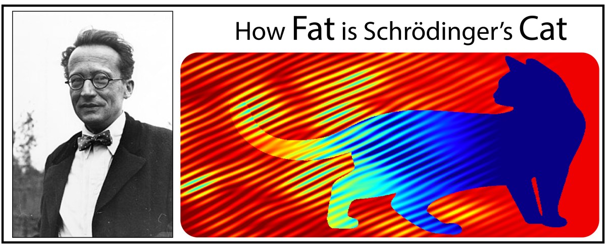
There is more than one absurdity hidden behind the gauzy clouds of quantum physics. No matter how hard the Ecclesiastes of the quantum canon have tried to hide them, the absurdities always tended to shine through. Niels Bohr, the high priest of the quantum, established the dogma in the raiment of the Copenhagen interpretation that became a windmill tilted at by the Don Quixote’s of physics. Surprisingly, two of the first to tilt at Copenhagen were also two of the founders of the field: Einstein and Schrödinger. Schrödinger created an absurdity—his “Cat”—that he thought would slay Bohr’s windmill, only to see it embraced by the enemy in its tiniest form, and then to grow ever larger until today some of the cat’s descendants are so fat they can be seen with the naked eye.
Einstein’s Spooky Action and Schrödinger’s Cat
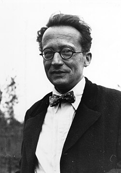
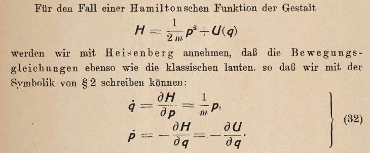
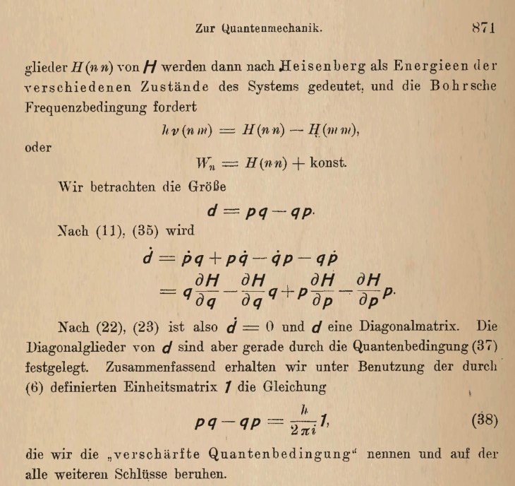
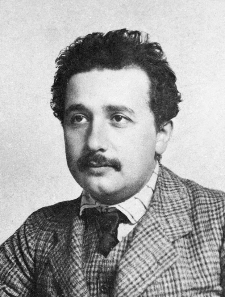
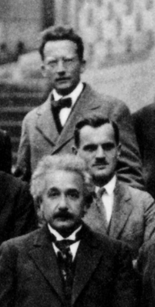
Albert Einstein and Erwin Schrödinger were founders of quantum physics. Einstein, on his part, blew past Planck by embracing quanta in the form of the quantum of light—the photon. Schrödinger, just as important, found the wave equation that governed the behavior of quantum particles. These two physicists believed that quantum dynamics should be just as deterministic as classical dynamics, and they pushed hard against Max Born and Niels Bohr and Werner Heisenberg who embraced the fundamental uncertainties of quantum measurement.
In the view of Einstein and Schrödinger, beginning in 1925, quantum mechanics had slowly veered off the tracks, and by 1935 they felt it had coagulated into a form that was both unrecognizable and unpalatable.
Einstein took the first pass, tilting at the nonlocal character of quantum physics that allowed a measurement at one location to determine the measurement at a distant location, no matter how far apart the two locations were. This is the famous “EPR Paradox”, named after the three authors of the paper published in the Physical Review in 1935 by Einstein, Podolsky and Rosen. Einstein called it “Spooky action at a distance.”
After reading the EPR paper, Schrödinger sent a congratulatory note to Einstein, applauding him on his clever thought experiment that showed one of the absurdities of quantum physics. This note launched an intense correspondence between the two physicists, as each complained to the other about the overbearing Copenhagen interpretation and about the indifference of a ballooning number of physicists who were happy to adopt Bohr’s attitudes without worrying about the underlying philosophical contradictions.
Inspired by his correspondence with Einstein, Schrödinger launched his own attack on Copenhagen. Where Einstein attacked the nonlocality of quantum phenomena, Schrödinger attacked the scale of quantum phenomena.
Schrödinger’s Cat
In late 1935, Schrödinger published a series of papers discussing the current situation in quantum mechanics [1]. Schrödinger had remained a realist. Although Born had established almost ten years before that the quantum wavefunction was not related to the physically real electron density, Schrödinger continued to ascribe to it a level of physical reality. To reduce the Copenhagen interpretation to absurdity, he took Bohr’s measurement argument to extremes.
Schrödinger proposed placing a cat in a sealed box with a radioactive substance known to have a half-life of an hour. If the particle decays, a Geiger counter in the box releases a hammer that smashes a vial of poison, killing the cat. At the end of an hour, the chance the cat is alive or dead is 50/50. In the Copenhagen interpretation, because all elements in the box consist of quantum mechanical wavefunctions, and no overt measurement is made, the cat must be in a quantum superposition of both alive and dead states. Now if an observer opens the box to look inside, the wavefunction of the cat collapses into one state or the other. To Schrödinger, such a state of affairs was absurd, clearly illustrating the limitations of the Copenhagen interpretation that required wavefunction superpositions to remain unmolested if no overt measurement takes place.
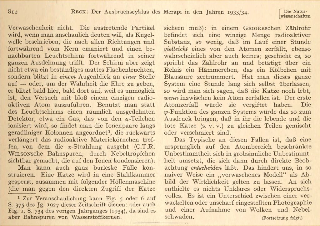
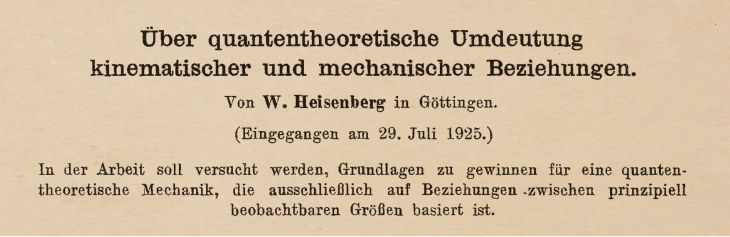
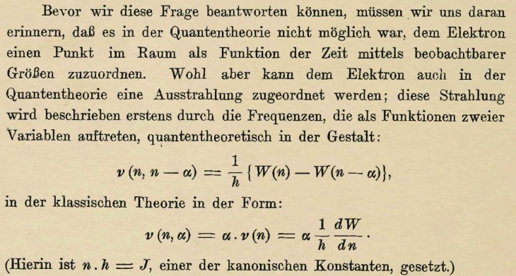
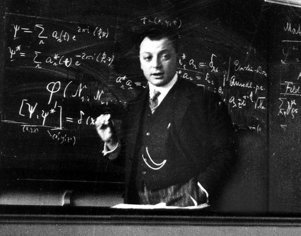
The translation of Schrödinger’s introduction of his cat (Fig. 2) is:
“One can even construct quite burlesque cases. A cat is penned up in a steel chamber, along with the following hellish machine (which must be secured against direct interference by the cat): in a Geiger counter, there is a tiny amount of radioactive substance, so little that in the course of an hour, perhaps one of the atoms decays, but also, with equal probability, perhaps none; if it happens, the counter tube responds and discharges through a relay a little hammer that shatters a small flask of prussic acid [hydrogen cyanide].
If one has left this entire system to itself for an hour, one would say that the cat still lives if no atom has decayed in the meantime. The first atomic decay would have poisoned it. The ψ-function of the entire system would express this by having in it the living and the dead cat (if I may be forgiven the expression) mixed or smeared out in equal parts.
The typical thing about these cases is that an uncertainty originally restricted to the atomic domain becomes transformed into macroscopic uncertainty, which can then be resolved by direct observation. This prevents us from so naively accepting a ‘blurred model’ as a representation of reality. In itself, it would contain nothing unclear or contradictory. There is a difference between a shaky or out-of-focus photograph and a snapshot of clouds and fog banks.”
The Schrödinger cat paradox became sensationally famous in ways that Schrödinger himself had not intended. He had fashioned the example to combat what he saw was an unrealistic acceptance of the Copenhagen interpretation of quantum mechanics. While succeeding in showing that quantum mechanics was bizarre, he had hoped to show that it was wrong, or at least missing something. To his chagrin, there was general acceptance of the dead-and-alive superposition, at least in principle. Schrödinger had called the mutual influence of quantum states upon each other as entanglement, and the word stuck. The discussions elicited by the cat paradox side-stepped the philosophical problems of quantum mechanics and focused instead on the physical differences between microscopic states, where quantum superposition held sway, versus macroscopic states, where classical physics emerges.
Today, the quantum/classical border is understood to be governed by decoherence. When a quantum system (with its well-defined superpositions) interacts with its environment, the internal quantum states become entangled with the environmental states, and the internal states lose their originally clean relationships, becoming fuzzy—less both “dead and alive” to become more “dead or alive”. By the simple combinatorics of large numbers, the bigger a quantum state is, the more avenues there are to interact with its environment, and the faster the effects of decoherence kick in. The question then shifts from whether a quantum cat can exist, to how large the quantum cat can become before decoherence gets too fast to capture the superposition.
Schrödinger’s Cat Grows Up
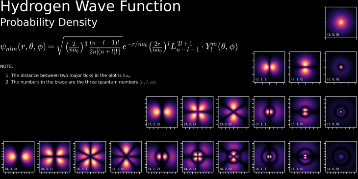
For the first several decades of its life, the size of Schrödinger’s cat was restricted to the quantum physics of fundamental particles, like electrons, or to electronic superpositions within atoms or molecules. These superpositions were not “spatial”—the two entities of the superposition were not occupying different parts of space. The electronic states of atoms could be in different orbitals that have different spatial distributions, but it is all one object.
This changed in 1974 when Italian physicists Pier Giorgio Merli, Gian Franco Missiroli, and Giulio Pozzi at the University of Bologna used the electron source of an electron microscope to send single electrons, one at a time, through a biprism acting as a double slit (like Young’s double slit experiment with light). This was the first time that the electron double-slit experiment was performed one electron at a time, and despite the fact that there was no “other” electron to interfer with, the experiment produced interference fringes. Each electron was in a superposition, taking both one path and the other, separated spatially by the two halves of the biprism. This was the first demonstration of Schrödinger’s cat as a spatial superposition.
This experiment was followed 15 years later by researchers at Hitachi in Japan who, in 1989, used a scintillator screen to watch the single electrons arrive one at a time, slowly building up the interference fringes first seen by the Italians.
Electrons interfering with themselves, by taking different spatial paths, still represents a tiny cat. Of the stable fundamental particles, electrons are the lightest (or the “smallest”). A more impressive cat might be constructed of an atom that is heavier and “larger” than an electron.
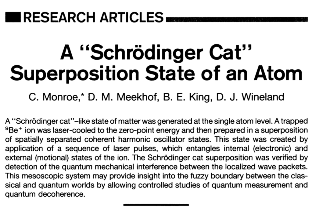
In 1996, Chris Monroe and David Wineland at JILA created a Schrödinger Cat superposition using a trapped Beryllium ion [2]. They coupled the internal electronic states to external motional states that allowed the ion to be prepared in a superposition of spatially separated states.
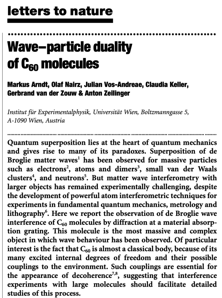
An even larger cat was demonstrated in 1999 by Anton Zeilinger‘s group in Vienna by creating a spatial quantum superposition using “Buckyballs” [3] that are C60 molecules. They used a thermal molecular beam at low flux levels that ensured that the average number of molecules transiting the experimental apparatus at a given time was less than one. One member of the group, Markus Arndt, has been “scaling up” the size of his cats into the range of thousands of atoms.
Schrödinger’s Cat Today
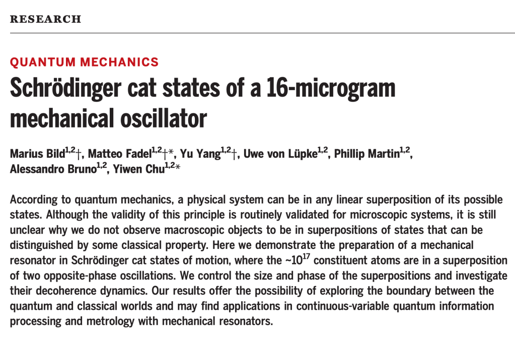
In the last 10 years, Schrödinger’s cat has grown to immense size. In 2023 a group at ETH in Zurick, Switzerland, put a “Fat Cat” 16-microgram mass [4] into a spatial superposition of two states of mechanical vibration. The mass contained approximately 1017 atoms (C60 has 60 atoms), which clearly brought quantum mechanics to the edge of the macroscopic world. It was shaped as a disc with a diameter of about 1 millimeter and a thickness of of 100 microns, large enough to be seen with the naked eye (before it is loaded into the ultra-low-temperature cryostat where it is hidden from probing eyes). The states experienced decoherence after about 40 microseconds, but this is a sufficiently long time for experimental probes to test its properties.
The 16-microgram mass experiment was macroscopic but still comprised a single object in two spatial modes. Therefore, by building on the C60 experiment of Markus Arndt, in early 2026 a matter wave interferometer measured the interference of large metal clusters of sodium [5] containing approximately 7000 atoms passing through a region of space that was macroscopically large relative to the size of the metal clusters. By some measure of “macroscopicity” this is the largest Quantum Cat to date.
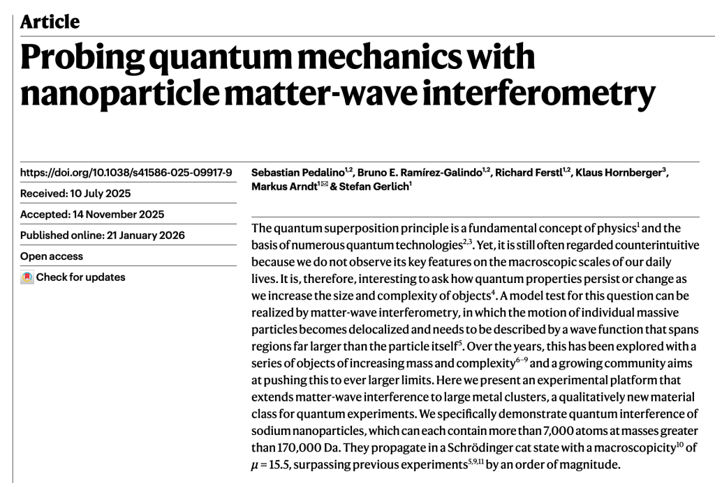
A simplified schematic of the Pedalino experiment is shown in Fig. 8. A nanoclusters with about 7000 sodium atoms comes from a source and moves towards a standing-wave laser beam. If the cluster moves into an antinode, then it is ionized and removed, but if it enters a node region, it remains neutral and passes through. This creates a spatial superposition of “locations” of the nanoparticle. This superposition creates quantum interference fringes on the far side of the diffraction grating.
The nanoparticle is about 10 nm in size, which is comparable to some biological macromolecules as well as viruses, raising the possibility that quantum cats may be constructed in the near future of biological matter. It may even become possible to produce quantum cats from living bacteria. Experimental groups continue to push the bounds of large quantum systems. This is of more than “academic” interest, because larger quantum superpositions with longer decoherence times can be enlisted as elements of quantum information systems such as quantum computers and quantum communication systems.
References
[1] Schrodinger, E. (1935). “The current situation in quantum mechanics.” Naturwissenschaften 23: 807-812.
[2] P.G. Merli, G.F. Missiroli, and G. Pozzi, “Electron interferometry with the Elmiskop 101 electron microscope,” Journal of Physics E: Scientific Instruments 7 (1974), 729–732
[3] C. Monroe et al. , A “Schrödinger Cat” Superposition State of an Atom. Science272,1131-1136(1996). DOI:10.1126/science.272.5265.1131
[4] Arndt, M., Nairz, O., Vos-Andreae, J. et al. Wave–particle duality of C60 molecules. Nature 401, 680–682 (1999). https://doi.org/10.1038/44348
[5] Marius Bild et al., Schrödinger cat states of a 16-microgram mechanical oscillator. Science380, 274-278(2023). DOI:10.1126/science.adf7553
[5] Pedalino, S., Ramírez-Galindo, B.E., Ferstl, R. et al. Probing quantum mechanics with nanoparticle matter-wave interferometry. Nature 649, 866–870 (2026). https://doi.org/10.1038/s41586-025-09917-9