
Gerardus Mercator was born in no-man’s land, in Flanders’ fields, caught in the middle between the Protestant Reformation and the Holy Roman Empire. In his lifetime, armies washed back and forth over the countryside, sacking cities and obliterating the inhabitants. At age 32 he was imprisoned by the Inquisition for heresy, though he had committed none, and languished for months as the authorities searched for the slimmest evidence against him. They found none and he was released, though several of his fellow captives—elite academicians of their day—met their ends burned at the stake or beheaded or buried alive. It was not an easy time to be a scholar, with you and your work under persistent attack by political zealots.
Mercator received the degree of Magister, the degree in medieval universities that is equivalent to a Doctor of Philosophy … and then took what today we would call a “gap year” to “find himself” …
Yet in the midst of this turmoil and destruction, Mercator created marvels. Originally trained for the Church, he was bewitched by cartography at a time when the known world was expanding rapidly after the discoveries of the New World. Though the cognoscenti had known that the Earth was spherical since long before the Greeks, everyone saw it as flat, including cartographers, who in practice had to render it on flat maps. When the world was local, flat maps worked well. But as the world became global, new cartography methods were needed to capture the sphere, and Mercator entered the profession at just the moment when cartography was poised for a revolution.
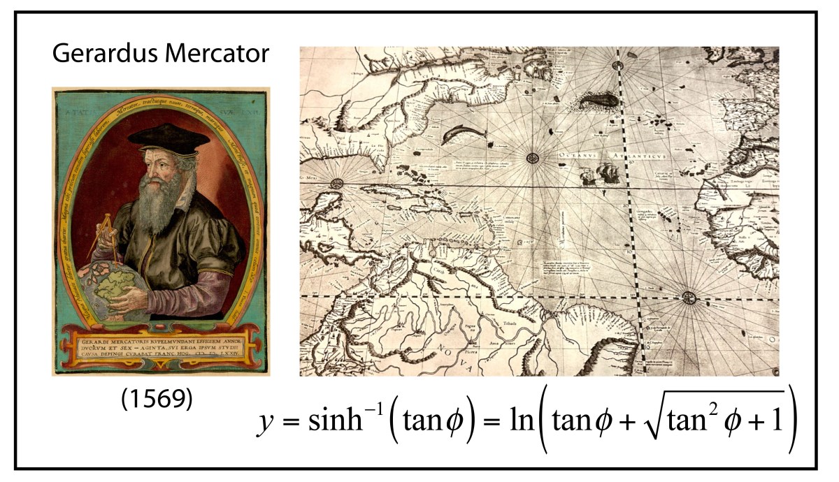
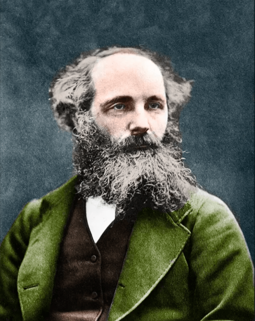
Gerardus Mercator
The life of Gerardus Mercator (1512 – 1594) spanned nearly the full 16th century. He was born 20 years after Colombus’ first voyage, and he died as Galileo began to study the law of fall, as Kepler began his study of planetary motion, and as Shakespeare began writing Romeo and Juliet. Mercator was born in the town of Rupelmonde, Flanders, outside of Antwerp in the southern part of the Netherlands ruled by Hapsburg Spain. His father was a poor shoemaker, but his uncle was an influential member of the clergy who paid for his nephew to attend a famous local school, in ‘s-Hertogenbosch, one where the humanist philosopher Erasmus (1466 – 1536) had attended several decades earlier.
Mercator entered the University of Leuven in 1530 in the humanities where his friends included Andreas Vesalius (the future famous anatomist) and Antoine Granvelle (who would become one of the most powerful Cardinals of the era). Mercator received the degree of Magister, the degree in medieval universities that is equivalent to a Doctor of Philosophy, in 1532, and then took what today we would call a “gap year” to “find himself” because he was having doubts about his faith and his future in the clergy. It was during his gap year that he was introduced to cartography by the Franciscan friar Franciscus Monachus (1490 – 1565) at the Mechelen monastery situated between Antwerp and Brussels.
Returning to the University of Leuven in 1534, he launched himself into the physical sciences of geography and mathematics, for which he had no training, but he quickly mastered them under the tutelage of the Dutch mapmaker Gemma Frisius (1508 – 1555) at the university. In 1537 Mercator completed his first map, a map of Palestine that received wide acclaim for its accuracy and artistry, and (more importantly) it sold well. He had found his vocation.
Early Cartography
Maps are among the oldest man-made textual artefacts, dating to nearly 7000 BCE, several millennia before the invention of writing itself. Knowing where things are, and where you are in relation to them, is probably the most important thing to remember in daily life. Texts are memory devices, and maps are the oldest texts.
The Alexandrian mathematician Claudius Ptolemy, around 150 CE, compiled a list of all the known world in his Geografia and drew up a map to accompany it. It survived through Arabic translation and became a fixture in early medieval Europe where it remained a record of virtually all that was known until Christopher Columbus ran into the Caribbean Islands in 1492 on his way to China. Maps needed to be redrawn.

The first map to show the new world was printed in 1500 by the Castillan navigator Juan de la Cosa, who had sailed with Columbus three times. His map included the explorations of John Cabot to the northern coasts.

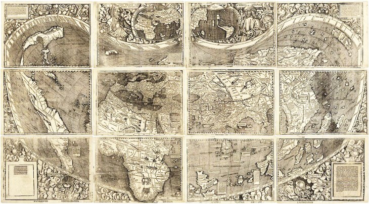
De la Cosa’s map was followed shortly by the world map of Martin Waldseemüller who named a small part of Brazil “America” in honor of Amerigo Vespucci who had just published an account of his adventures along the coasts of the new lands.
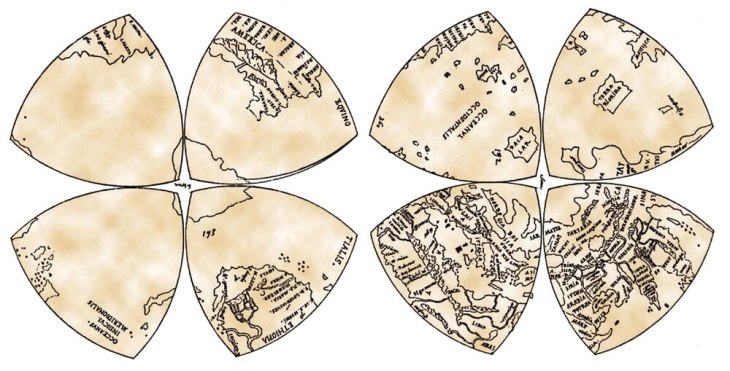
Leonardo da Vinci went further and created an eight-octant map of the globe around 1514, calling the entire new landmass “America”, expanding on Waldseemüller’s use of the name beyond merely Brazil.
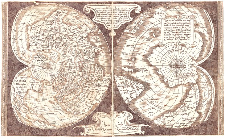
In 1538, just a year after his success with his Palastine map, Mercator created a map of the world that showed for the first time the separation of the Americas into two continents, the North and the South, expanding the name “America” to its full modern extent.
These maps by the early cartographers were not functional maps for navigation, but were large, sometimes many feet across, meant to be displayed to advantage on the spacious walls in the rooms of the rich and famous. On the other hand, since the late Middle Ages, there had been a long-standing tradition of map making among navigators whose lives depended on the utility and accuracy of their maps. These navigational charts were called Portolan Charts, meaning literally charts of ports or harbors. They carried sheaves of straight lines representing courses of constant magnetic bearing, meaning that the angle between the compass needle and the direction of the boat stayed constant. These are called rhumb lines, and they allowed ships to navigate between two known points beyond the sight of land. The importance of rhumb lines far surpassed the use of decorative maps. Mercator knew this, and for his next world map, he decided to give it rhumb lines that spanned the globe. The problem was how to do it.

A Conformal Projection
Around the time that Mercator was bursting upon the cartographic scene, a Portuguese mathematician, Pedro Nunes, was studying courses of constant bearing upon a spherical globe. These are mathematical paths on the sphere that were later called loxodromes, but over short distances, they corresponded to the rhumb line.
Thirty years later, Mercator had become a master cartographer, creating globes along with scientific instruments and maps. His globes were among the most precise instruments of their day, and he learned how to draw accurate loxodromes, following the work of Nunes. On a globe, these lines became “curly cues” as they approached a Pole of the sphere, circling around the Pole in ever tighter circles that defied mathematical description (until many years later when Thomas Harriot showed they were logarithmic spirals). Yet Mercator was a master draftsman, and he translated the curved loxodromes on the globe into straight lines on a world map. What he discovered was a projection in which all lines of Longitude and all lines of Meridian were straight lines, as were all courses of constant bearing. He completed his map in 1569, explicitly hawking its utility as a map that could be used on a global scale just as Portolan charts had been used in the Mediterranean.

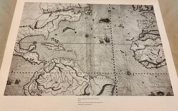
Mercator in 1569 was already established and famous and an old hand at making maps, yet even he was impressed by the surprising unity of his discovery. Today, the Mercator projection is called a conformal map, meaning that all angles among intersecting lines on the globe are conserved in the planar projection, explaining the linear longitudes, latitudes and rhumbs.
The Geometry of Gerhardus Mercator
Mercator’s new projection is a convenient exercise in differential geometry. Begin with the transformation from spherical coordinates to Cartesian coordinates
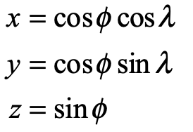
where λ is the longitude and φ is the latitude. The Jacobian matrix is
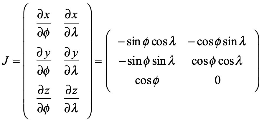
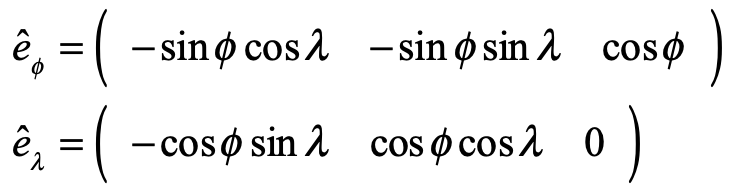
Taking the transpose, and viewing each row as a new vector
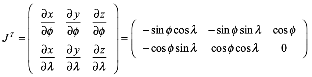
creates the basis vectors of the spherical surface
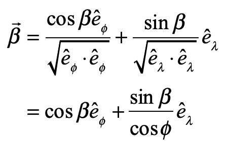
A unit vector with constant heading at angle β is expressed in the new basis vectors as
and the path length and arc length along a constant-bearing path are related as
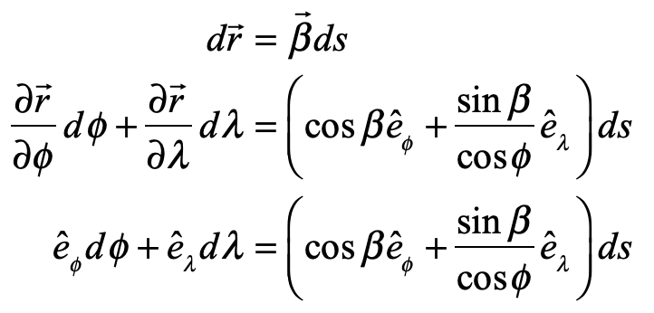
Equating common coefficients of the basis vectors gives
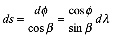
which is solved to yield the ordinary differential equation
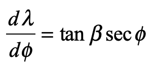
This is integrated as
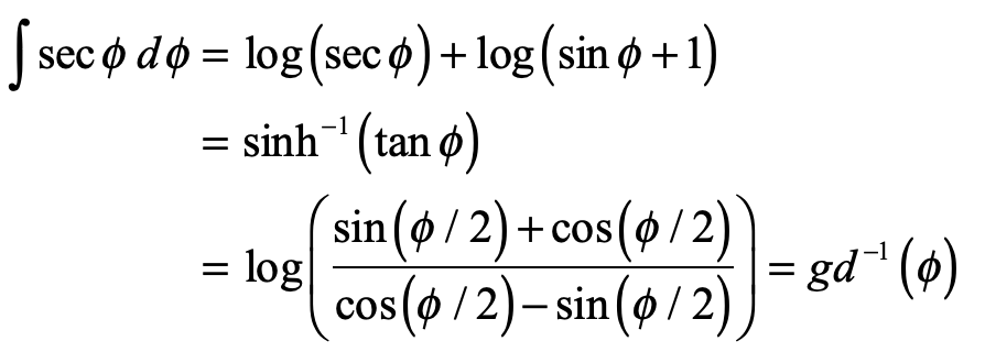
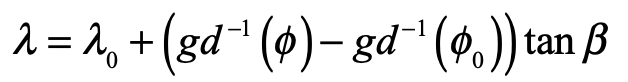
which is a logarithmic spiral. The special function is called “the inverse Gundermannian”. The longitude λ as a function of the latitude φ is solved as
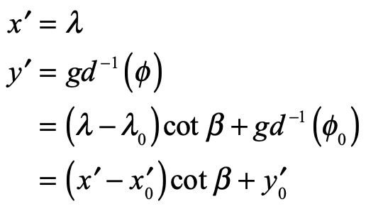
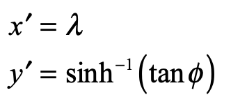
To generate a Mercator rhumb, we only need to go back to a new set of Cartesian coordinates on a flat map
It is interesting to compare the Mercator projection to a conical projection onto a cylinder touching the sphere at its equator where the Mercator projection is
while the conical projection onto the cylinder is
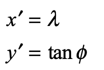
Clearly, the two projections are essentially the same around the Equator, but deviate exponentially approaching the Poles.
The Mercator projection has the conformal advantage, but it also has the disadvantage that landmasses at increasing latitude increase in size relative to their physical size on the glove. Therefore, Greenland looks as big as Africa on a Mercator projection, while it is in fact only about the size of Texas. The exaggerated sizes of countries in the upper latitudes (like the USA and Europe) relative to tropical countries near the equator has been viewed as creating an unfair psychological bias of first-world countries over third-world countries. For this reason, Mercator projections are virtually never used today, with other map projections that retain relative sizes being now the most common.
References
Crane, N. (2002), Mercator: The Man who Mapped the Planet, Weidenfeld & Nicolson, London.
Kythe, P. K. (2019), Handbook of Conformal Mappings and Applications, CRC Press.
Monmonier, M. S. (2004), Rhumb Lines and Map Wars: A Social History of the Mercator Projection, University of Chicago Press.
Snyder, J. P. (2002), Flattening the earth: Two thousand years of map projections, 5. ed ed., The University of Chicago Press, Chicago
Taylor, A. (2004), The World of Gerard Mercator: The Mapmaker Who Revolutionized Geography, Walker & Company, New York.


.jpg)