
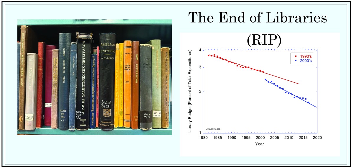
Beware!
If you love books, don’t read this post. Close the tab and look away from the second burning of the Library of Alexandria.
If you love books, then run to your favorite library (if it is still there), and take out every book you have ever thought of. Fill your rooms and offices with checked-out books, the older the better, and never, ever, return them. Keep clicking on RENEW, for as long as they let you.
The librarians had paved paradise and put up a parking lot.
If you love books, the kind of rare valueless books on topics only you care about, then Librarians—the former Jedi gatekeepers of knowledge—have turned to the dark side, deaccessioning the unpopular books in the stacks, pulling their loan cards like tomb stones, shipping the books away in unmarked boxes like body bags to large warehouses to be sold for pennies—and you may never see them again.
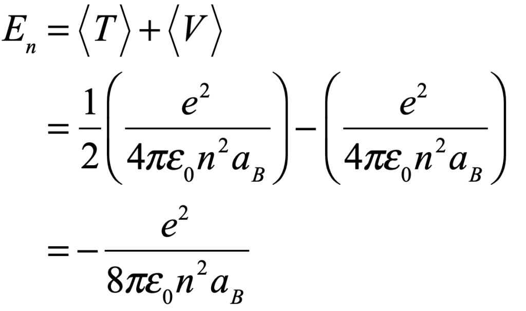
The End of Physics
Just a few years ago my university, with little warning and no consultation with the physics faculty, closed the heart and soul of the Physics Department—our Physics Library. It was a bright warm space where we met colleagues, quietly discussing deep theories, a place to escape for a minute or two, or for an hour, to browse a book picked from the shelf of new acquisitions—always something unexpected you would never think to search for online. But that wasn’t the best part.
The best part was the three floors above, filled with dark and dusty stacks that seemed to rise higher than the building itself. This was where you found the gems—books so old or so arcane that when you pulled them from the shelf to peer inside, they sent you back, like a time machine, to an era when physicists thought differently—not wrong, but differently. And your understanding of your own physics was changed, seen with a longer lens, showing you things that went deeper than you expected, and you emerged from the stacks a changed person.
And then it was gone.
They didn’t even need the space. At a university where space is always in high demand, and turf wars erupt between departments who try to steal space in each other’s buildings, the dark cavernous rooms of the ex-physics library stood empty for years as the powers at be tried to figure out what to do with it.

So, I determined to try to understand how a room that stood empty would be more valuable to a university than a room full of books. What I discovered was at the same time both mundane and shocking. Mundane, because it delves into the rules and regulations that govern how universities function. Shocking, because it is a betrayal of the very mission of universities and university libraries.
How to Get Accreditation Without Really Trying
Little strikes fear in the heart of a college administrator like the threat of losing accreditation. Accreditation is the stamp of approval that drives sales—sales of slots in the freshman incoming class. Without accreditation, a college is nothing more than a bunch of buildings housing over-educated educators. But with accreditation, the college has a mandate to educate and has the moral authority to mold the minds of the next generation.
In times past—not too long past—let’s say up to the end of the last millennium, to receive accreditation, a college or university would need to spend something around 3% of its operating budget on the upkeep of its libraries. For a moderate-sized university library system, this was on the order of $20M per year. The requirement was a boon to the librarians who kept a constant lookout for new books to buy to populate the beloved “new acquisitions” shelf.
Librarians reveled in their leverage over the university administrators: buy books or lose accreditation. It was a powerful negotiating position to be in. But all that changed in the early 2000’s. Universities are always strapped for cash (despite tuition increases rising at two-times the rate of inflation) and the librarian’s $20M cash cow was a tempting target. Universities are also powerful, running their billion-dollar-a-year operations, and they lobbied the very organizations that give the accreditations, convincing them to remove the requirement for the minimum library budget. After all, in the digital world, who needs expensive buildings filled with books, the vast majority of which never get checked out?
The Deaccessioning Wars: Double Fold
Twenty some years ago, a bibliovisionary by the name of Nicholson Baker recognized the book armegeddon of his age and wrote about it in Double Fold: Libraries and the Assault on Paper (Vintage Books/Random House, 2001). Libraries everywhere were in the midst of an orgy of deaccessioning. To deaccession a book means to remove it from the card catalog (an anachronism) and ship it off to second-hand book dealers. But it was worse than that. Many of the books, as well as rare journals and rarer newspapers, were being “guillotined” by cutting out each page and scanning it into some kind of visual/digital format before pitching all the pages into the recycle bin. The argument in favor of guillotining is that all paper must eventually decay to dust (a false assumption).
The way to test whether a book, or a newspaper, is on its way to dissolution is to do the double fold test on a corner of a page. You fold the corner over then back the other way—double fold—and repeat. The double-fold number of a book is how many double folds it takes for the little triangular piece to fall off. Any number less than a selected threshold gives a librarian carte blanch to deaccession the book, and maybe to guillotine it, regardless of how the book may be valued.
Librarians generally hate Baker’s little book Double Fold because deaccessioning is always a battle. Given finite shelf space, for every new acquisition, something old needs to go. How do you choose? Any given item might be valued by someone, so an objective test that removes all shades of gray is the double-fold. It is a blunt instrument, one that Nicholas Baker abhorred, but it does make room for the new—if that is all that a university library is for.
As an aside, as I write this blog, my university library, which does not own a copy of Double Fold, and through which I had to request a copy via Interlibrary Loan (ILL), is threatening me with punitive action if I don’t relinquish it because it is a few weeks overdue. If my library had actually owned a copy, I could have taken it out and kept it on my office shelf for years, as long as I kept hitting that “renew” button on the library page. (On the other hand, my university does own a book by the archivist Cox who wrote a poorly argued screed to try to refute Baker.)
The End of Deep Knowledge
Baker is already twenty years out of date, although his message is more dire now than ever. In his day, deaccessioning was driven by that problem of finite shelf space—one book out for one book in. Today, when virtually all new acquisitions are digital, that argument is moot. Yet the current rate at which books are disappearing from libraries, and libraries themselves are disappearing from campuses, is nothing short of cataclysmic, dwarfing the little double-fold problem that Baker originally railed against.
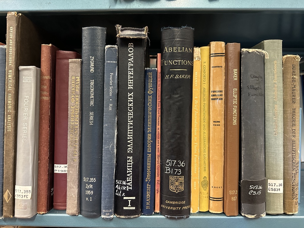
My university used to have a dozen specialized libraries scattered across campus, with the Physics Library one of them. Now there are maybe three in total. One of those is the Main Library which was an imposing space filled with the broadest range of topics and a truly impressive depth of coverage. You could stand in front of any stack and find beautifully produced volumes (with high-quality paper that would never fail the double fold test) on beautifully detailed topics, going as deep as you could wish to the very foundations of knowledge.
I am a writer of the history of science and technology, and as I write, I often will form a very specific question about how a new idea emerged. What was its context? How did it break free of old mindsets? Why was it just one individual who saw the path forward? What made them special?
My old practice was to look up a few books in the library catalog that may or may not have the kinds of answers I was looking for, then walk briskly across campus to the associated library (great for exercise and getting a break from my computer). I would scan across the call numbers on the spines of the books until I found the book I sought—and then I would step back and look at the whole stack.
Without fail, I would find gems I never knew existed, sometimes three, four or five shelves away from the book I first sought. They were often on topics I never would have searched online. And to find those gems, I would take down book after book, scanning them quickly before returning them to the shelf (yes, I know, re-shelving is a no-no, but the whole stack would be emptied if I followed the rules) and moving to the next—something you could never do online. In ten minutes, or maybe half an hour if I lost track of time, I would have three or four books crucial to my argument in the crook of my arm, ready to walk down the stairs to circulation to take them out. Often, the book that launched my search was not even among them.
I thought that certainly this main library was safe, and I was looking forward to years ahead of me, even past retirement, buried in its stacks, sleuthing out the mysteries of the evolution of knowledge.
And then it was gone.
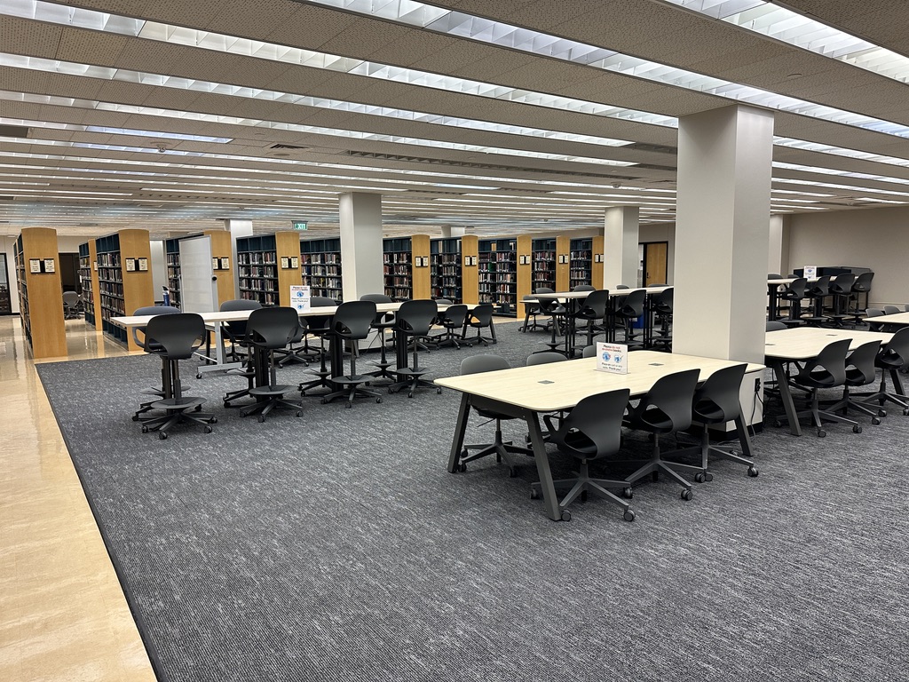
Not the building or the space—they were still there. But the rows upon rows of stacks had been replaced with study space that students didn’t even need. Once again, empty space was somehow more valuable to the library than having that space filled with books. The librarians had paved paradise and put up a parking lot. To me, it was like a death in the family.
Why not bulldoze Williamsburg, Virginia, after digital capture? Why not burn the USS Constitution in Boston Bay after photographing it? Why not flatten the Alamo?
I recently looked up a book that was luckily still available at the Main Library in one of its few remaining stacks. So I went to find it. The shelves all around it were only about two-thirds filled, the wide gaps looking like abandoned store-fronts in a failing city. And what books did remain were the superficial ones—the ones that any undergrad might want to take out to get an overview of some well-worn topic (which they could probably just get on Wikipedia). All the deep knowledge (which Wikipedia will never see) was gone.
I walked out with exactly the one book I had gone to find—not a single surprising gem to accompany it. But the worst part is the opportunity cost: I will never know what I had failed to discover!

Shrinking Budgets and Predatory Publishers
So why is a room that stands empty more valuable to a university than a room full of books? Here are the mundane and shocking answers.
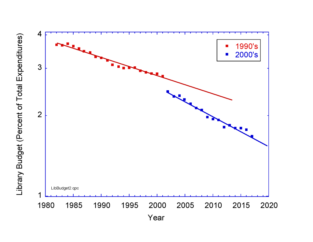
On the one hand, library budgets are under assault. The following figure shows library expenditures as a percentage of total university expenditures averaged for 40 major university libraries tabulated by the ARL (Association of Research Libraries) from 1982 to 2017. There is an exponential decrease in the library budget as a function of year, with a break right around 2000-2001 when accreditation was no longer linked to library expenditures. Then the decay accelerated.
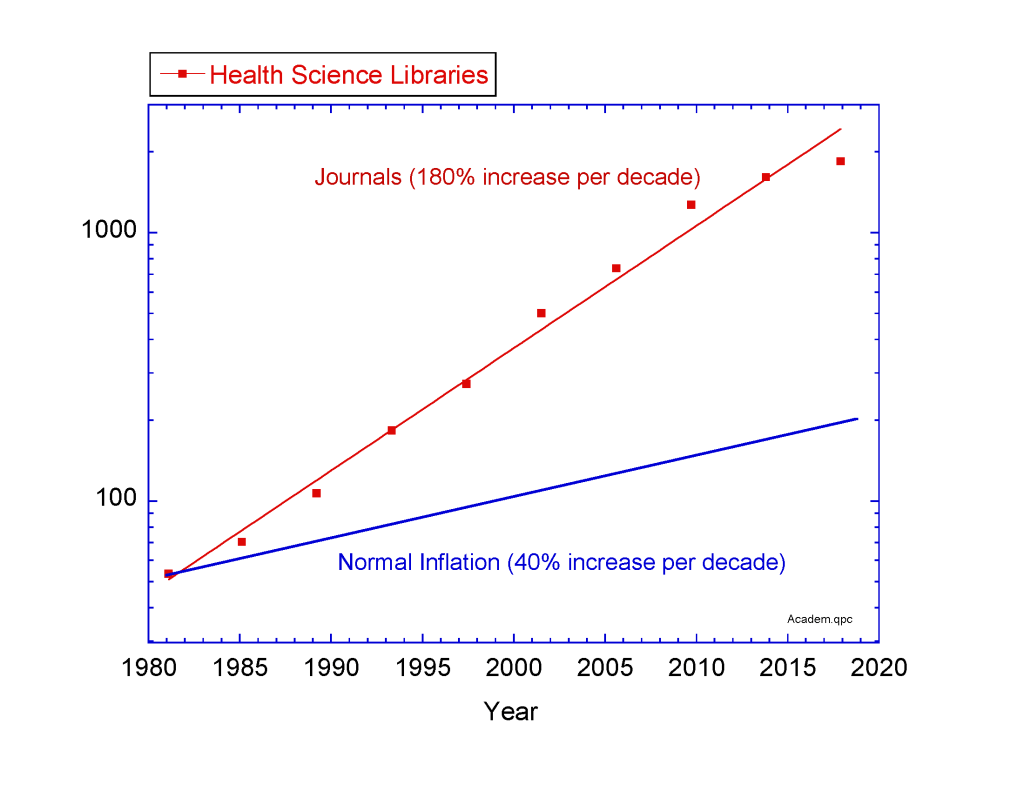
Combine decreasing rates of library funding with predatory publishers, and the problem is compounded. The following figure shows the increasing price of journal subscriptions that universities must pay relative to the normal inflation rate. The journal publishers are increasing their prices exponentially, tripling the cost each decade, a rate that erodes library budgets even more. Therefore, it is tempting to say that librarians don’t actually hate books, but are victims of bad economics. But that is the mundane answer.
The shocking answer is that modern librarians find books to be anachronistic. The new hires are by and large “digital librarians” who are focused on providing digital content to serve students who have become much more digital, especially after Covid. There is also a prevailing opinion among university librarians that students want more space to study, hence the removal of stacks to be replaced by soft chairs and open study spaces.
And that is the betrayal. The collections of deep knowledge, which are unique and priceless and irreplaceable, were replaced by generic study space that could be put anywhere at any time, having no intrinsic value.
You can argue that I still have access to the knowledge because of Interlibrary Loan (ILL). But ILL only works if other libraries have yet to remove the book. What happens when every library thinks that some other library has the book, and so they throw their own copy out? At some point that volume will have vanished from all collections and that will be the end of it.
Or you can argue that I can find the book digitally scanned on Internet Archive or Google Books. But I have already found situations where special folio pages, the very pages that I needed to make my argument, had failed to be reproduced in the digital versions. And the books were too rare to be allowed to go through ILL. So I was stuck.
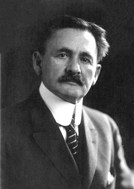
(By the way, this was a rare copy of the works of Francois Arago. In my book Interference: Optical Interferometry and the Scientists who Tamed Light (Oxford University Press, 2023), I make the case that it was Arago who invented the first interferometer in 1816 long before Albert Michelson’s work in 1880. But for the final smoking gun, to prove my case, I needed that folio page which took Herculean efforts to eventually track down. Our Physics Library had the book in its stacks just a decade ago, and I could have just walked upstairs from my office to look at it. Where it is now is anyone’s guess.)
But digital scans are no substitute for the real thing. To hold an old volume in your hands, run off the printing press when the author was still alive, and filled with scribbled notes in the margins by your colleagues from years past, is to commune with history. Why not bulldoze Williamsburg, Virginia, after digital capture? Why not burn the USS Constitution in Boston Bay after photographing it? Why not flatten the Alamo? When you immerse yourself in these historical settings, you gain an understanding that is deeper than possible by browsing an article on Wikipedia.
People react to the real, like real books. Why take that away?
Acknowledgements: This post is the product of several discussions with my brother, James Nolte, a retired reference librarian. He was an early developer of digital libraries, working at Clarkson University in Potsdam, NY in the mid 1980’s. But like Frankenstein, he sometimes worries about the consequences of his own creation.


