February 5, 2025September 3, 2025 by David D. Nolte

A Short History of Neural Networks

History of Dynamics
ai, Artificial Intelligence, Attention mechanism, convolutional neural network, Deep Learning, History of Physics, Hopfield network, Machine Learning, neural networks, Neurodynamics, Nonlinear Dynamics, recurrent neural network, technology, van der Pol oscillator
1 Comment

When it comes to questions about the human condition, the question of intelligence is at the top. What is the origin of our intelligence? How intelligent are we? And how intelligent can we make other things…things like artificial neural networks?

This is a short history of the science and technology of neural networks, not just artificial neural networks but also the natural, organic type, because theories of natural intelligence are at the core of theories of artificial intelligence. Without understanding our own intelligence, we probably have no hope of creating the artificial type.

Ramon y Cajal (1888): Visualizing Neurons

The story begins with Santiago Ramon y Cajal (1853 – 1934) who received the Nobel Prize in physiology in 1906 for his work illuminating natural neural networks. He built on work by Camillo Golgi, using a stain to give intracellular components contrast [1], and then went further to developed his own silver emulsions like those of early photography (which was one of his hobbies). Cajal was the first to show that neurons were individual constituents of neural matter and that their contacts were sequential: axons of sets of neurons contacted the dendrites of other sets of neurons, never axon-to-axon or dendrite-to-dendrite, to create a complex communication network. This became known as the neuron doctrine, and it is a central idea of neuroscience today.

*Fig. 1 One of Cajal’s published plates demonstrating neural synapses. From Link.*

McCulloch and Pitts (1943): Mathematical Models

In 1941, Warren S. McCulloch (1898–1969) arrived at the Department of Psychiatry at the University of Illinois at Chicago where he met with the mathematical biology group at the University of Chicago led by Nicolas Rashevsky (1899–1972), widely acknowledged as the father of mathematical biophysics in the United States.

An itinerant member of Rashevsky’s group at the time was a brilliant, young and unusual mathematician, Walter Pitts (1923– 1969). He was not enrolled as a student at Chicago, but had simply “showed up” one day as a teenager at Rashevsky’s office door. Rashevsky was so impressed by Pitts that he invited him to attend the group meetings, and Pitts became interested in the application of mathematical logic to biological information systems.

When McCulloch met Pitts, he realized that Pitts had the mathematical background that complemented his own views of brain activity as computational processes. Pitts was homeless at the time, so McCulloch invited him to live with his family, giving the two men ample time to work together on their mutual obsession to provide a logical basis for brain activity in the way that Turing had provided it for computation.

McCulloch.and.Pitts Download

McColloch and Pitts simplified the operation of individual neurons to their most fundamental character, envisioning a neural computing unit with multiple inputs (received from upstream neurons) and a single on-off output (sent to downstream neurons) with the additional possibility of feedback loops as downstream neurons fed back onto upstream neurons. They also discretized the dynamics in time, using discrete logic and time-difference equations, succeeding in devising a logical structure with rules and equations for the general operation of nets of neurons. They published their results a 1943 in the paper titled “A logical calculus of the ideas immanent in nervous activity,” [2] introducing computational language and logic to neuroscience. Their simplified neural unit became the basis for discrete logic, picked up a few years later by von Neumann as an elemental example of a logic gate upon which von Neumann began constructing the theory and design of the modern electronic computer.

*Fig. 2 The only figure in McCulloch and Pitt’s “Logical Calculus”.*

Donald Hebb (1949): Hebbian Learning

The basic model for learning and adjustment of synaptic weights among neurons was put forward in 1949 by the physiological psychologist Donald Hebb (1904-1985) of McGill University in Canada in a book titled The Organization of Behavior [3].

In Hebbian learning, an initially untrained network consists of many neurons with many synapses having random synaptic weights. During learning, a synapse between two neurons is strengthened when both the pre-synaptic and post-synaptic neurons are firing simultaneously. In this model, it is essential that each neuron makes many synaptic contacts with other neurons because it requires many input neurons acting in concert to trigger the output neuron. In this way, synapses are strengthened when there is collective action among the neurons. The synaptic strengths are therefore altered through a form of self-organization. A collective response of the network strengthens all those synapses that are responsible for the response, while the other synapses that do not contribute, weaken. Despite the simplicity of this model, it has been surprisingly robust, standing up as a general principle for the training of artificial neural networks.

*Fig. 3. A Figure from Hebb’s textbook on psychology (1958). From Link.*

Hodgkin and Huxley (1952): Neuron Transporter Models

Alan Hodgkin (1914 – 1998) and Andrew Huxley (1917 – 2012) were English biophysicists who received the 1963 Nobel Prize in physiology for their work on the physics behind neural activation. They constructed a differential equation for the spiking action potential for which their biggest conceptual challenge was the presence of time delays in the voltage signals that were not explained by linear models of the neural conductance. As they began exploring nonlinear models, using their experiments to guide the choice of parameters, they settled on a dynamical model in a four-dimensional phase space. One dimension was voltage, while another was inhibitory current. The two remaining dimensions were sodium and potassium conductances, which they had determined were the major ions participating in the generation and propagation of the action potential. The nonlinear conductances of their model described the observed time delays and captured the essential neural behavior of the fast spike followed by a slow recovery. Huxley solved the equations on a hand-cranked calculator, taking over three months of tedious cranking to plot the numerical results.

*Fig. 4 The Hodgkin-Huxley model of the neuron, including capacitance C, voltage V and bias current I along with the conductances of potassium (K), sodium (Na) and Lithium (L) channels.*

Hodgkin and Huxley published [4] their measurements and their model (known as the Hodgkin-Huxley model) in a series of six papers in 1952 that led to an explosion of research in electrophysiology, for which Hodgkin and Huxley won the 1963 Nobel Prize in physiology or medicine. The four-dimensional Hodgkin–Huxley model stands as a classic example of the power of phenomenological modeling when combined with accurate experimental observation. Hodgkin and Huxley were able to ascertain not only the existence of ion channels in the cell membrane, but also their relative numbers, long before these molecular channels were ever directly observed using electron microscopes. The Hodgkin–Huxley model lent itself to simplifications that could capture the essential behavior of neurons while stripping off the details.

Frank Rosenblatt (1958): The Perceptron

Frank Rosenblatt (1928–1971) had a PhD in psychology from Cornell University and was in charge of the cognitive systems section of the Cornell Aeronautical Laboratory (CAL) located in Buffalo, New York. He was tasked with fulfilling a contract from the Navy to develop an analog image processor. Drawing from the work of McCulloch and Pitts, his team constructed a software system and then constructed a hardware model that adaptively updated the strength of the inputs, that they called neural weights, as it was trained on test images. The machine was dubbed the Mark I Perceptron, and its announcement in 1958 created a small media frenzy [5]. A New York Times article reported the perceptron was “the embryo of an electronic computer that [the navy] expects will be able to walk, talk, see, write, reproduce itself and be conscious of its existence.”

rosenblatt-1957 Download

The perceptron had a simple architecture, with two layers of neurons consisting of an input layer and a processing layer, and it was programmed by adjusting the synaptic weights to the inputs. This computing machine was the first to adaptively learn its functions, as opposed to following predetermined algorithms like digital computers. It seemed like a breakthrough in cognitive science and computing, as trumpeted by the New York Times. But within a decade, the development had stalled because the architecture was too restrictive.

Fig. 5 Frank Rosenblatt with his Perceptron. From Link.

Richard Fitzhugh and Jin-Ichi Nagumo (1961): Neural van der Pol Oscillators

In 1961 Richard FitzHugh (1922–2007), a neurophysiology researcher at the National Institute of Neurological Disease and Blindness (NINDB) of the National Institutes of Health (NIH), created a surprisingly simple model of the neuron that retained only a third order nonlinearity, just like the third-order nonlinearity that Rayleigh had proposed and solved in 1883, and that van der Pol extended in 1926. Around the same time that FitzHugh proposed his mathematical model [6], the electronics engineer Jin-Ichi Nagumo (1926-1999) in Japan created an electronic diode circuit with an equivalent circuit model that mimicked neural oscillations [7]. Together, this work by FitzHugh and Nagumo led to the so-called FitzHugh–Nagumo model. The conceptual importance of this model is that it demonstrated that the neuron was a self-oscillator, just like a violin string or wheel shimmy or the pacemaker cells of the heart. Once again, self-oscillators showed themselves to be common elements of a complex world—and especially of life.

*Fig. 6 The FitzHugh-Nagumo model of the neuron simplifies the Hodgkin-Huxley model from four dimensions down to two dimensions of voltage V and channel activation n.*

Fitzhugh_1961 Download

John Hopfield (1982): Spin Glasses and Recurrent Networks

John Hopfield (1933–) received his PhD from Cornell University in 1958, advised by Al Overhauser in solid state theory, and he continued to work on a broad range of topics in solid state physics as he wandered from appointment to appointment at Bell Labs, Berkeley, Princeton, and Cal Tech. In the 1970s Hopfield’s interests broadened into the field of biophysics, where he used his expertise in quantum tunneling to study quantum effects in biomolecules, and expanded further to include information transfer processes in DNA and RNA. In the early 1980s, he became aware of aspects of neural network research and was struck by the similarities between McColloch and Pitts’ idealized neuronal units and the physics of magnetism. For instance, there is a type of disordered magnetic material called a spin glass in which a large number of local regions of magnetism are randomly oriented. In the language of solid-state physics, one says that the potential energy function of a spin glass has a large number of local minima into which various magnetic configurations can be trapped. In the language of dynamics, one says that the dynamical system has a large number of basins of attraction [8].

Hopfieldpnas00447-0135 Download

The Parallel Distributed Processing Group (1986): Backpropagation

David Rumelhart, a mathematical psychologist at UC San Diego, was joined by James McClelland in 1974 and then by Geoffrey Hinton in 1978 to become what they called the Parallel Distributed Processing (PDP) group. The central tenets of the PDP framework they developed were: 1) processing is distributed across many semi-autonomous neural units, that 2) learn by adjusting the weights of their interconnections based on the strengths of their signals (i.e., Hebbian learning), whose memories and behaviors are 3) an emergent property of the distributed learned weights.

PDP was an exciting framework for artificial intelligence, and it captured the general behavior of natural neural networks, but it had a serious problem: How could all of the neural weights be trained?

In 1986, Rumelhart and Hinton with the mathematician Ronald Williams developed a mathematical procedure for training neural weights called error backpropagation [9]. The idea is actually very simple: create a mean squared error of the response of a neural network compared to an ideal response, then tweak one of the neural weights and see if the error increases or decreases. If the error decreases, keep the tweak for that weight and move to the next, working iteratively, tweak by tweak, to minimize the mean squared error. In this way, large numbers of neural weights can be adjusted as the network is trained to perform a specified task.

Error backpropagation has come a long way from that early 1986 paper, and it now lies at the core of the AI revolution we are experiencing today as tens of millions of neural weights are trained on massive datasets.

Rumelhart323533a0 Download

Yann LeCun (1989): Convolutional Neural Networks

In 1988, I was a new post-doc at AT&T Bell Labs at Holmdel, New Jersey fresh out of my PhD in physics from Berkeley. Bell Labs liked to give its incoming employees inspirational talks and tours of their facilities, and one of the tours I took was of the neural network lab run by Lawrence Jackel that was working on computer recognition of zip-code digits. The team’s new post-doc, arriving at Bell Labs the same time as me, was Yann LeCun. It is very possible that the demo our little group watched was run by him, or at least he was there, but at the time he was a nobody, so even if I had heard his name, it wouldn’t have meant anything to me.

Fast forward to today, and Yann LeCun’s name is almost synonomous with AI. He is the Chief AI Scientist at Facebook and his google scholar page reports that he gets 50,000 citations per year.

LeCun is famous for developing the convolutional neural network (CNN) in work that he published from Bell Labs in 1989 [10]. It is a biomimetic neural network that takes its inspiration from the receptive fields of the neural networks in the retina. What you think you see, when you look at something, is actually reconstructed by your brain. Your retina is a neural processor with receptive fields that are a far cry from one-to-one. Most prominent in the retina are center-surround fields, or kernels, that respond to the derivatives of the focused image instead of the image itself. It’s the derivatives that are sent up your optic neuron to your brain which then reconstructs the image. It works as a form of image compression so that broad uniform areas in an image are reduced to its edges.

LeCun.neco.1989.1.4.541 Download

The convolutional neural network works in the same way, it’s just engineered specifically to produce compressed and multiscale codes that capture broad areas as well as the fine details of an image. By constructing many different “kernel” operators at many different scales, it creates a set of features that capture the nuances of the image in quantitative form that is then processed by training neural weights in downstream neural networks.

Fig. 7 Example of a receptive field of a CNN. The filter is the kernel (in this case a discrete 3×3 Laplace operator) that is stepped sequentially across the image field to produce the Laplacian feature map of the original image. One feature map for every different kernel becomes the input for the next level of kernels in a hierarchical scaling structure.

Geoff Hinton (2006): Deep Belief

It seems like Geoff Hinton has had his finger in almost every pie when it comes to how we do AI today. Backpropagation? Geoff Hinton. Rectified Linear Units? Geoff Hinton. Boltzmann Machines? Geoff Hinton. t-SNE? Geoff Hinton. Dropout regularization? Geoff Hinton. AlexNet? Geoff Hinton. The 2024 Nobel Prize in Physics? Geoff Hinton! He may not have invented all of these, but he was in the midst of it all.

Hinton received his PhD in Artificial Intelligence (ar rare field at the time) from the University of Edinburgh in 1978 after which he joined the PDP group at UCSD (see above) as a post-doc. After a time at Carnegie-Mellon, he joined the University of Toronto, Canada, in 1987 where he established one of the leading groups in the world on neural network research. It was from here that he launched so many of the ideas and techniques that have become the core of deep learning.

A central idea of deep learning came from Hinton’s work on Boltzmann Machines that learn statistical distributions of complex data. This type of neural network is known as an energy-based model, similar to a Hopfield network, and it has strong ties to the statistical mechanics of spin-glass systems. Unfortunately, it is a bitch to train! So Hinton simplified it into a Restricted Boltzmann Machine (RBM) that was much more tractable and layers of RBMs could be stacked into “Deep Belief Networks” [11] that had a hierarchical structure that allowed the neural nets to learn layers of abstractions. These were among the first deep networks that were able to do complex tasks at the level of human capabilities (and sometimes beyond).

The breakthrough that propelled Geoff Hinton to world-wide acclaim was the success of AlexNet, a neural network constructed by his graduate student Alex Krizhevsky at Toronto in 2012 consisting of 650,000 neurons with 60 million parameters that were trained using two early Nvidia GPUs. It won the ImageNet challenge that year, enabled by its deep architecture and representing a marked advancement that has been proceeding unabated today.

AttentionIsAllYouNeed2017 Download

Deep learning is now the rule in AI, supported by the Attention mechanism and Transformers that underpin the large language models, like ChatGPT and others, that are poised to disrupt all the legacy business models based on the previous silicon revolution of 50 years ago.

References

[1] Ramón y Cajal S. (1888). Estructura de los centros nerviosos de las aves. Rev. Trim. Histol. Norm. Pat. 1, 1–10.

[2] McCulloch, W.S. and W. Pitts, A Logical Calculus of the Ideas Immanent in Nervous Activity. Bull. Math. Biophys., 1943. 5: p. 115.

[3] Hebb, D. O. (1949). The Organization of Behavior: A Neuropsychological Theory. New York: Wiley and Sons. ISBN 978-0-471-36727-7 – via Internet Archive.

[4] Hodgkin AL, Huxley AF (August 1952). “A quantitative description of membrane current and its application to conduction and excitation in nerve”. The Journal of Physiology. 117 (4): 500–44.

[5] Rosenblatt, Frank (1957). “The Perceptron—a perceiving and recognizing automaton”. Report 85-460-1. Cornell Aeronautical Laboratory.

[6] FitzHugh, Richard (July 1961). “Impulses and Physiological States in Theoretical Models of Nerve Membrane”. Biophysical Journal. 1 (6): 445–466.

[7] Nagumo, J.; Arimoto, S.; Yoshizawa, S. (October 1962). “An Active Pulse Transmission Line Simulating Nerve Axon”. Proceedings of the IRE. 50 (10): 2061–2070.

[8] Hopfield, J. J. (1982). “Neural networks and physical systems with emergent collective computational abilities”. Proceedings of the National Academy of Sciences. 79 (8): 2554–2558.

[9] Rumelhart, D.E. et al. Nature 323, 533-536 (1986).

[10] Y. LeCun, B. Boser, J. S. Denker, D. Henderson, R. E. Howard, W. Hubbard and L. D. Jackel: Backpropagation Applied to Handwritten Zip Code Recognition, Neural Computation, 1(4):541–551, Winter 1989.

[11] G. E. Hinton, S. Osindero, and Y. W. Teh, “A fast learning algorithm for deep belief nets,” Neural Computation 18, 1527-1554 (2006).

Read more in Books by David D. Nolte at Oxford University Press

December 11, 2024September 5, 2025 by David D. Nolte

100 Years of Quantum Physics: Pauli’s Exclusion Principle (1924)

One hundred years ago this month, in December 1924, Wolfgang Pauli submitted a paper to Zeitschrift für Physik that provided the final piece of the puzzle that connected Bohr’s model of the atom to the structure of the periodic table. In the process, he introduced a new quantum number into physics that governs how matter as extreme as neutron stars, or as perfect as superfluid helium, organizes itself.

He was led to this crucial insight, not by his superior understanding of quantum physics, which he was grappling with as much as Bohr and Born and Sommerfeld were at that time, but through his superior understanding of relativistic physics that convinced him that the magnetism of atoms in magnetic fields could not be explained through the orbital motion of electrons alone.

Encyclopedia Article on Relativity

Bored with the topics he was being taught in high school in Vienna, Pauli was already reading Einstein on relativity and Emil Jordan on functional analysis before he arrived at the university in Munich to begin studying with Arnold Sommerfeld. Pauli was still merely a student when Felix Klein approached Sommerfeld to write an article on relativity theory for his Encyclopedia of Mathematical Sciences. Sommerfeld by that time was thoroughly impressed with Pauli’s command of the subject and suggested that he write the article.

PauliRelativity Download

Pauli’s encyclopedia article on relativity expanded to 250 pages and was published in Klein’s fifth volume in 1921 when Pauli was only 21 years old—just 5 years after Einstein had published his definitive work himself! Pauli’s article is still considered today one of the clearest explanations of both special and general relativity.

Pauli’s approach established the methodical use of metric space concepts that is still used today when teaching introductory courses on the topic. This contrasts with articles written only a few years earlier that seem archaic by comparison—even Einstein’s paper itself. As I recently read through his article, I was struck by how similar it is to what I teach from my textbook on modern dynamics to my class at Purdue University for junior physics majors.

Anomalous Zeeman Effect

In 1922, Pauli completed his thesis on the properties of water molecules and began studying a phenomenon known as the anomalous Zeeman effect. The Zeeman effect is the splitting of optical transitions in atoms under magnetic fields. The electron orbital motion couples with the magnetic field through a semi-classical interaction between the magnetic moment of the orbital and the applied magnetic field, producing a contribution to the energy of the electron that is observed when it absorbs or emits light.

The Bohr model of the atom had already concluded that the angular momentum of electron orbitals was quantized into integer units. Furthermore, the Stern-Gerlach experiment of 1922 had shown that the projection of these angular momentum states onto the direction of the magnetic field was also quantized. This was known at the time as “space quantization”. Therefore, in the Zeeman effect, the quantized angular momentum created quantized energy interactions with the magnetic field, producing the splittings in the optical transitions.

File:Breit-rabi-Zeeman-en.svg — Fig. 2 The magnetic Zeeman splitting of Rb-87 from the weak field to the strong-field (Pachen-Back) effect

So far so good. But then comes the problem with the anomalous Zeeman effect.

In the Bohr model, all angular momenta have integer values. But in the anomalous Zeeman effect, the splittings could only be explained with half integers. For instance, if total angular momentum were equal to one-half, then in a magnetic field it would produce a “doublet” with +1/2 and -1/2 space quantization. An integer like L = 1 would produce a triplet with +1, 0, and -1 space quantization. Although doublets of the anomalous Zeeman effect were often observed, half-integers were unheard of (so far) in the quantum numbers of early quantum physics.

But half integers were not the only problem with “2”s in the atoms and elements. There was also the problem of the periodic table. It, too, seemed to be constructed out of “2”s, multiplying a sequence of the difference of squares.

The Difference of Squares

The difference of squares has a long history in physics stretching all the way back to Galileo Galilei who performed experiments around 1605 on the physics of falling bodies. He noted that the distance traveled in successive time intervals varied as the difference 1² – 0² = 1, then 2²-1² = 3, then 3²-2² = 5, then 4²-3² = 7 and so on. In other words, the distances traveled in each successive time interval varied as the odd integers. Galileo, ever the astute student of physics, recognized that the distance traveled by an accelerating body in a time t varied as the square of time t². Today, after Newton, we know that this is simply the dependence of distance for an accelerating body on the square of time s = (1/2)gt².

By early 1924 there was another law of the difference of squares. But this time the physics was buried deep inside the new science of the elements, put on graphic display through the periodic table.

The periodic table is constructed on the difference of squares. First there is 2 for hydrogen and helium. Then another 2 for lithium and beryllium, followed by 6 for B, C, N, O, F and Ne to make a total of 8. After that there is another 8 plus 10 for the sequence of Sc, Ti, V, Cr, Mn, Fe, Co, Ni, Cu and Zn to make a total of 18. The sequence of 2-8-18 is 2•1² = 2, 2•2² = 8, 2•3² = 18 for the sequence 2n².

Why the periodic table should be constructed out of the number 2 times the square of the principal quantum number n was a complete mystery. Sommerfeld went so far as to call the number sequence of the periodic table a “cabalistic” rule.

The Bohr Model for Many Electrons

It is easy to picture how confusing this all was to Bohr and Born and others at the time. From Bohr’s theory of the hydrogen atom, it was clear that there were different energy levels associated with the principal quantum number n, and that this was related directly to angular momentum through the motion of the electrons in the Bohr orbitals.

But as the periodic table is built up from H to He and then to Li and Be and B, adding in successive additional electrons, one of the simplest questions was why the electrons did not all reside on the lowest energy level? But even if that question could not be answered, there was the question of why after He the elements Li and Be behaved differently than B, N, O and F, leading to the noble gas Ne. From normal Zeeman spectroscopy as well as x-ray transitions, it was clear that the noble gases behaved as the core of succeeding elements, like He for Li and Be and Ne for Na and Mg.

To grapple with all of this, Bohr had devised a “building up” rule for how electrons were “filling” the different energy levels as each new electron of the next element was considered. The noble-gas core played a key role in this model, and the core was also assumed to be contributing to both the normal Zeeman effect as well as the anomalous Zeeman effect with its mysterious half-integer angular momenta.

But frankly, this core model was a mess, with ad hoc rules on how the additional electrons were filling the energy levels and how they were contributing to the total angular momentum.

This was the state of the problem when Pauli, with his exceptional understanding of special relativity, began to dig deep into the problem. Since the Zeeman splittings were caused by the orbital motion of the electrons, the strongly bound electrons in high-Z atoms would be moving at speeds near the speed of light. Pauli therefore calculated what the systematic effects would be on the Zeeman splittings as the Z of the atoms got larger and the relativistic effects got stronger.

He calculated this effect to high precision, and then waited for Landé to make the measurements. When Landé finally got back to him, it was to say that there was absolutely no relativistic corrections for Thallium (Z = 90). The splitting remained simply fixed by the Bohr magneton value with no relativistic effects.

Pauli had no choice but to reject the existing core model of angular momentum and to ascribe the Zeeman effects to the outer valence electron. But this was just the beginning.

Pauli’s Breakthrough

https://onionesquereality.wordpress.com/wp-content/uploads/2012/07/wolfgang-pauli.jpg — Fig. 5 Wolfgang Pauli [Image]

By November of 1924 Pauli had concluded, in a letter to Landé

“In a puzzling, non-mechanical way, the valence electron manages to run about in two states with the same k but with different angular momenta.”

And in December of 1924 he submitted his work on the relativistic effects (or lack thereof) to Zeitschrift für Physik,

“From this viewpoint the doublet structure of the alkali spectra as well as the failure of Larmor’s theorem arise through a specific, classically non-describable sort of Zweideutigkeit (two-foldness) of the quantum-theoretical properties of the valence electron. (Pauli, 1925a, pg. 385)

Around this time, he read a paper by Edmund Stoner in the Philosophical Magazine of London published in October of 1924. Stoner’s insight was a connection between the number of states observed in a magnetic field and the number of states filled in the successive positions of elements in the periodic table. Stoner’s insight led naturally to the 2-8-18 sequence for the table, although he was still thinking in terms of the quantum numbers of the core model of the atoms.

This is when Pauli put 2 plus 2 together: He realized that the states of the atom could be indexed by a set of 4 quantum numbers: n-the principal quantum number, k1-the angular momentum, m1-the space quantization number, and a new fourth quantum number m2 that he introduced but that had, as yet, no mechanistic explanation. With these four quantum numbers enumerated, he then made the major step:

It should be forbidden that more than one electron, having the same equivalent quantum numbers, can be in the same state. When an electron takes on a set of values for the four quantum numbers, then that state is occupied.

This is the Exclusion Principle: No two electrons can have the same set of quantum numbers. Or equivalently, no electron state can be occupied by two electrons.

Fig. 6 Level filling for Krypton using the Pauli Exclusion Principle

Today, we know that Pauli’s Zweideutigkeit is electron spin, a concept first put forward in 1925 by the American physicist Ralph Kronig and later that year by George Uhlenbeck and Samuel Goudsmit.

The “Famous” Pauli Exclusion Paper Download

And Pauli’s Exclusion Principle is a consequence of the antisymmetry of electron wavefunctions first described by Paul Dirac in 1926 after the introduction of wavefunctions into quantum theory by Erwin Schrödinger earlier that year.

Timeline:

1845 – Faraday effect (rotation of light polarization in a magnetic field)

1896 – Zeeman effect (splitting of optical transition in a magnetic field)

1897 – Anomalous Zeeman effect (half-integer splittings)

1902 – Lorentz and Zeeman awarded Nobel prize (for electron theory)

1921 – Paschen-Back effect (strong-field Zeeman effect)

1922 – Stern-Gerlach (space quantization)

1924 – de Broglie matter waves

1924 – Bose statistics of photons

1924 – Stoner (conservation of number of states)

1924 – Pauli Exclusion Principle

References:

E. C. Stoner (Philosophical Magazine, 48 [1924], 719) Issue 286 October 1924

M. Jammer, The conceptual development of quantum mechanics (Los Angeles, Calif.: Tomash Publishers, Woodbury, N.Y. : American Institute of Physics, 1989).

M. Massimi, Pauli’s exclusion principle: The origin and validation of a scientific principle (Cambridge University Press, 2005).

Pauli, W. Über den Einfluß der Geschwindigkeitsabhängigkeit der Elektronenmasse auf den Zeemaneffekt. Z. Physik 31, 373–385 (1925). https://doi.org/10.1007/BF02980592

Pauli, W. (1925). “Über den Zusammenhang des Abschlusses der Elektronengruppen im Atom mit der Komplexstruktur der Spektren”. Zeitschrift für Physik. 31 (1): 765–783

Read more in Books by David Nolte at Oxford University Press

September 25, 2024September 5, 2025 by David D. Nolte

Edward Purcell: From Radiation to Resonance

As the days of winter darkened in 1945, several young physicists huddled in the basement of Harvard’s Research Laboratory of Physics, nursing a high field magnet to keep it from overheating and dumping its field. They were working with bootstrapped equipment—begged, borrowed or “stolen” from various labs across the Harvard campus. The physicist leading the experiment, Edward Mills Purcell, didn’t even work at Harvard—he was still on the payroll of the Radiation Laboratory at MIT, winding down from its war effort on radar research for the military in WWII, so the Harvard experiment was being done on nights and weekends.

Just before Christmas, 1945, as college students were fleeing campus for the first holiday in years without war, the signal generator, borrowed from a psychology lab, launched an electromagnetic pulse into simple paraffin—and disappeared! It had been absorbed by the nuclear spins of the copious number of hydrogen nuclei (protons) in the wax.

The experiment was simple, unfunded, bootstrapped—and it launched a new field of physics that ultimately led to magnetic resonance imaging (MRI) that is now the workhorse of 3D medical imaging.

This is the story, in Purcell’s own words, of how he came to the discovery of nuclear magnetic resonance in solids, for which he was awarded the Nobel Prize in Physics in 1952.

Early Days

Edward Mills Purcell (1912 – 1997) was born in a small town in Illinois, the son of a telephone businessman, and some of his earliest memories were of rummaging around in piles of telephone equipment—wires and transformers and capacitors. He especially like the generators:

“You could always get plenty of the bell-ringing generators that were in the old telephones, which consisted of a series of horseshoe magnets making the stator field and an armature that was wound with what must have been a mile of number 39 wire or something like that… These made good shocking machines if nothing else.”

His science education in the small town was modest, mostly chemistry, but he had a physics teacher, a rare woman at that time, who was open to searching minds. When she told the students that you couldn’t pull yourself up using a single pulley, Purcell disagreed and got together with a friend:

“So we went into the barn after school and rigged this thing up with a seat and hooked the spring scales to the upgoing rope and then pulled on the downcoming rope.”

The experiment worked, of course, with the scale reading half the weight of the boy. When they rushed back to tell the physics teacher, she accepted their results immediately—demonstration trumped mere thought, and Purcell had just done his first physics experiment.

However, physics was not a profession in the early 1920’s.

“In the ’20s the idea of chemistry as a science was extremely well publicized and popular, so the young scientist of shall we say 1928 — you’d think of him as a chemist holding up his test tube and sighting through it or something…there was no idea of what it would mean to be a physicist.

The name Steinmetz was more familiar and exciting than the name Einstein, because Steinmetz was the famous electrical engineer at General Electric and was this hunchback with a cigar who was said to know the four-place logarithm table by heart.”

Purdue University and Prof. Lark-Horowitz

Purcell entered Purdue University in the Fall of 1929. The University had only 4500 students who paid $50 a year to attend. He chose a major in electrical engineering, because

“Being a physicist…I don’t remember considering that at that time as something you could be…you couldn’t major in physics. You see, Purdue had electrical, civil, mechanical and chemical engineering. It had something called the School of Science, and you could graduate, having majored in science.”

But he was drawn to physics. The Physics Department at Purdue was going through a Renaissance under the leadership of its new department head Prof. Lark-Horovitz

“His [Lark-Horovitz] coming to Purdue was really quite important for American physics in many ways… It was he who subsequently over the years brought many important and productive European physicists to this country; they came to Purdue, passed through. And he began teaching; he began having graduate students and teaching really modern physics as of 1930, in his classes.”

Purcell attended Purdue during the early years of the depression when some students didn’t have enough money to find a home:

“People were also living down there in the cellar, sleeping on cots in the research rooms, because it was the Depression and some of the graduate students had nowhere else to live. I’d come in in the morning and find them shaving.”

Lark-Horovitz was a demanding department chair, but he was bringing the department out of the dark ages and into the modern research world.

“Lark-Horovitz ran the physics department on the European style: a pyramid with the professor at the top and everybody down below taking orders and doing what the professor thought ought to be done. This made working for him rather difficult. I was insulated by one layer from that because it was people like Yearian, for whom I was working, who had to deal with the Lark. “

Hubert Yearian had built a 20-kilovolt electron diffraction camera, a Debye-Scherrer transmission camera, just a few years after Davisson and Germer had performed the Nobel-prize winning experiment at Bell Labs that proved the wavelike nature of electrons. Purcell helped Yearian build his own diffraction system, and recalled:

“When I turned on the light in the dark room, I had Debye-Scherrer rings on it from electron diffraction — and that was only five years after electron diffraction had been discovered. So it really was right in the forefront. And as just an undergraduate, to be able to do that at that time was fantastic.”

Purcell graduated from Purdue in 1933 and from contacts through Lark-Horovitz he was able to spend a year in the physics department at Karlsruhe in Germany. He returned to the US in 1934 to enter graduate scool in physics at Harvard, working under Kenneth Bainbridge. His thesis topic was a bit of a bust, a dusty old problem in classical electrostatics that was a topic far older than the electron diffraction he worked on at Purdue. But it was enough to get him his degree in 1938, and he stayed on at Harvard as a faculty instructor until the war broke out.

Radiation Laboratory, MIT

In the Fall at the end of 1940 the Radiation Lab at MIT was launched and began vacuuming up all the unattached physicists in the United States, and Purcell was one of them. The radiation lab also vacuumed up some of the top physicists in the country, like Isidor Rabi from Columbia, to supervise the growing army of scientists that were committed to the war effort—even before the US was in the war.

“Our mission was to make a radar for a British night fighter using 10-centimeter magnetron that had been discovered at Birmingham.”

This research turned Purcell and his cohort into experts in radio-frequency electronics and measurement. He worked closely with Rabi (Nobel Prize 1944) and Norman Ramsey (Nobel Prize 1989) and Jerrold Zacharias, who were in the midst of measuring resonances in molecular beams. The names at the Rad Lab was like reading a Who’s Who of physics at that time:

“And then there was the theoretical group, which was also under Rabi. Most of their theory was concerned with electromagnetic fields and signal to noise, things of that sort. George Uhlenbeck was in charge of it for quite a long time, and Bethe was in it for a while; Schwinger was in it; Frank Carlson; David Saxon, now president of the University of California; Goudsmit also.”

Nuclear Magnetic Resonance

The research by Rabi had established the physics of resonances in molecular beams, but there were serious doubts that such phenomena could exist in solids. This became one of the Holy Grails of physics, with only a few physicists across the country with the skill and understanding to make a try to observe it in the solid state.

Many of the physicists at the Rad Lab were wondering what they should do next, after the war was over.

“Came the end of the war and we were all thinking about what shall we do when we go back and start doing physics. In the course of knocking around with these people, I had learned enough about what they had done in molecular beams to begin thinking about what can we do in the way of resonance with what we’ve learned. And it was out of that kind of talk that I was struck with the idea for what turned into nuclear magnetic resonance.”

“Well, that’s how NMR started, with that idea which, as I say, I can trace back to all those indirect influences of talking with Rabi, Ramsey and Zacharias, thinking about what we should do next.

“We actually did the first NMR experiment here [Harvard], not at MIT. But I wasn’t officially back. In fact, I went around MIT trying to borrow a magnet from somebody, a big magnet, get access to a big magnet so we could try it there and I didn’t have any luck. So I came back and talked to Curry Street, and he invited us to use his big old cosmic ray magnet which was out in the shed. So I didn’t ask anybody else’s permission. I came back and got the shop to make us some new pole pieces, and we borrowed some stuff here and there. We borrowed our signal generator from the Psycho Acoustic Lab that Smitty Stevens had. I don’t know that it ever got back to him. And some of the apparatus was made in the Radiation Lab shops. Bob Pound got the cavity made down there. They didn’t have much to do — things were kind of closing up — and so we bootlegged a cavity down there. And we did the experiment right here on nights and week-ends.

This was in December, 1945.

“Our first experiment was done on paraffin, which I bought up the street at the First National store between here and our house. For paraffin we thought we might have to deal with a relaxation time as long as several hours, and we were prepared to detect it with a signal which was sufficiently weak so that we would not upset the spin temperature while applying the r-f field. And, in fact, in the final time when the experiment was successful, I had been over here all night … nursing the magnet generator along so as to keep the field on for many hours, that being in our view a possible prerequisite for seeing the resonances. Now, it turned out later that in paraffin the relaxation time is actually 10^-4 seconds. So I had the magnet on exactly 10⁸ times longer than necessary!

The experiment was completed just before Christmas, 1945.

E. M. Purcell, H. C. Torrey, and R. V. Pound, “RESONANCE ABSORPTION BY NUCLEAR MAGNETIC MOMENTS IN A SOLID,” Physical Review 69, 37-38 (1946).

“But the thing that we did not understand, and it gradually dawned on us later, was really the basic message in the paper that was part of Bloembergen’s thesis … came to be known as BPP (Bloembergen, Purcell and Pound). [This] was the important, dominant role of molecular motion in nuclear spin relaxation, and also its role in line narrowing. So that after that was cleared up, then one understood the physics of spin relaxation and understood why we were getting lines that were really very narrow.”

Diagram of the microwave cavity filled with paraffin.

This was the discovery of nuclear magnetic resonance (NMR) for which Purcell shared the 1952 Nobel Prize in physics with Felix Bloch.

David D. Nolte is the Edward M. Purcell Distinguished Professor of Physics and Astronomy, Purdue University. Sept. 25, 2024

References and Notes

• The quotes from EM Purcell are from the “Living Histories” interview in 1977 by the AIP.

• K. Lark-Horovitz, J. D. Howe, and E. M. Purcell, “A new method of making extremely thin films,” Review of Scientific Instruments 6, 401-403 (1935).

• E. M. Purcell, H. C. Torrey, and R. V. Pound, “RESONANCE ABSORPTION BY NUCLEAR MAGNETIC MOMENTS IN A SOLID,” Physical Review 69, 37-38 (1946).

• National Academy of Sciences Biographies: Edward Mills Purcell

July 24, 2024September 5, 2025 by David D. Nolte

The Vital Virial of Rudolph Clausius: From Stat Mech to Quantum Mech

I often joke with my students in class that the reason I went into physics is because I have a bad memory. In biology you need to memorize a thousand things, but in physics you only need to memorize 10 things … and you derive everything else!

Of course, the first question they ask me is “What are those 10 things?”.

That’s a hard question to answer, and every physics professor probably has a different set of 10 things. Obviously, energy conservation would be first on the list, followed by other conservation laws for various types of momentum. Inverse-square laws probably come next. But then what? What do you need to memorize to be most useful when you are working out physics problems on the back of an envelope, when your phone is dead, and you have no access to your laptop or books?

One of my favorites is the Virial Theorem because it rears its head over and over again, whether you are working on problems in statistical mechanics, orbital mechanics or quantum mechanics.

The Virial Theorem

The Virial Theorem makes a simple statement about the balance between kinetic energy and potential energy (in a conservative mechanical system). It summarizes in a single form many different-looking special cases we learn about in physics. For instance, everyone learns early in their first mechanics course that the average kinetic energy <T> of a mass on a spring is equal to the average potential energy <V>. But this seems different than the problem of a circular orbit in gravitation or electrostatics where the average kinetic energy is equal to half the average potential energy, but with the opposite sign.

Yet there is a unity to these two—it is the Virial Theorem:

for cases where the potential energy V has power law dependence V ≈ rⁿ. The harmonic oscillator has n = 2, leading to the well-known equality between average kinetic and potential energy as

The inverse square force law has a potential that varies with n = -1, leading to the flip in sign. For instance, for a circular orbit in gravitation, it looks like

and in electrostatics it looks like

where a is the radius of the orbit.

Yet orbital mechanics is hardly the only place where the Virial Theorem pops up. It began its life with statistical mechanics.

Rudolph Clausius and his Virial Theorem

The pantheon of physics is a somewhat exclusive club. It lets in the likes of Galileo, Lagrange, Maxwell, Boltzmann, Einstein, Feynman and Hawking, but it excludes many worthy candidates, like Gilbert, Stevin, Maupertuis, du Chatelet, Arago, Clausius, Heaviside and Meitner all of whom had an outsized influence on the history of physics, but who often do not get their due. Of this later group, Rudolph Clausius stands above the others because he was an inventor of whole new worlds and whole new terminologies that permeate physics today.

Within the German Confederation dominated by Prussia in the mid 1800’s, Clausius was among the first wave of the “modern” physicists who emerged from new or reorganized German universities that integrated mathematics with practical topics. Carl Neumann at Königsberg, Carl Gauss and Max Weber at Göttingen, and Hermann von Helmholtz at Berlin were transforming physics from a science focused on pure mechanics and astronomy to one focused on materials and their associated phenomena, applying mathematics to these practical problems.

Clausius was educated at Berlin under Heinrich Gustav Magnus beginning in 1840, and he completed his doctorate at the University of Halle in 1847. His doctoral thesis on light scattering in the atmosphere represented an early attempt at treating statistical fluctuations. Though his initial approach was naïve, it helped orient Clausius to physics problems of statistical ensembles and especially to gases. The sophistication of his physics matured rapidly and already in 1850 he published his famous paper Über die bewegende Kraft der Wärme, und die Gesetze, welche sich daraus für die Wärmelehre selbst ableiten lassen (About the moving power of heat and the laws that can be derived from it for the theory of heat itself).

This was the fundamental paper that overturned the archaic theory of caloric, which had assumed that heat was a form of conserved quantity. Clausius proved that this was not true, and he introduced what are today called the first and second laws of thermodynamics. This early paper was one in which he was still striving to simplify thermodynamics, and his second law was mostly a qualitative statement that heat flows from higher temperatures to lower. He refined the second law four years later in 1854 with Über eine veranderte Form des zweiten Hauptsatzes der mechanischen Wärmetheorie (On a modified form of the second law of the mechanical theory of heat). He gave his concept the name Entropy in 1865 from the Greek word τροπη (transformation or change) with a prefix similar to Energy.

Clausius was one of the first to consider the kinetic theory of heat where heat was understood as the average kinetic energy of the atoms or molecules that comprised the gas. He published his seminal work on the topic in 1857 expanding on earlier work by Augustus Krönig. Maxwell, in turn, expanded on Clausius in 1860 by introducing probability distributions. By 1870, Clausius was fully immersed in the kinetic theory as he was searching for mechanical proofs of the second law of thermodynamics. Along the way, he discovered a quantity based on action-reaction pairs of forces that was related to the kinetic energy.

At that time, kinetic energy was often called vis viva, meaning “living force”. The singular of force (vis) had a plural (virias), so Clausius—always happy to coin new words—called the action-reaction pairs of forces the virial, and hence he proved the Virial Theorem.

The argument is relatively simple. Consider the action of a single molecule of the gas subject to a force F that is applied reciprocally from another molecule. Also, for simplicity consider only a single direction in the gas. The change of the action over time is given by the derivative

The average over all action-reaction pairs is

but by the reciprocal nature of action-reaction pairs, the left-hand side balances exactly to zero, giving

This expression is expanded to include the other directions and to all N bodies to yield the Virial Theorem

where the sum is over all molecules in the gas, and Clausius called the term on the right the Virial.

An important special case is when the force law derives from a power law

Then the Virial Theorem becomes (again in just one dimension)

This is often the most useful form of the theorem. For a spring force, it leads to <T> = <V>. For gravitational or electrostatic orbits it is <T> = -1/2<V>.

The Virial in Astrophysics

Clausius originally developed the Virial Theorem for the kinetic theory of gases, but it has applications that go far beyond. It is already useful for simple orbital systems like masses interacting through central forces, and these can be scaled up to N-body systems like star clusters or galaxies.

Star clusters are groups of hundreds or thousands of stars that are gravitationally bound. Such a cluster may begin in a highly non-equilibrium configuration, but the mutual interactions among the stars causes a relaxation to an equilibrium configuration of positions and velocities. This process is known as Virialization. The time scale for virializaiton depends on the number of stars and on the initial configuration, such as whether there is a net angular momentum in the cluster.

A gravitational simulation of 700 stars is shown in Fig. 2. The stars are distributed uniformly with zero velocities. The cluster collapses under gravitational attraction, rebounds and approaches a steady state. The Virial Theorem applies at long times. The simulation assumed all motion was in the plane, and a regularization term was added to the gravitational potential to keep forces bounded.

Simulation of the virial theorem for a star cluster with kinetic and potential energy graphs — Fig. 2 A numerical example of the Virial Theorem for a star cluster of 700 stars beginning in a uniform initial state, collapsing under gravitational attraction, rebounding and then approaching a steady state. The kinetic energy and the potential energy of the system satisfy the Virial Theorem at long times.

The Virial in Quantum Physics

Quantum theory holds strong analogs to classical mechanics. For instance, the quantum commutation relations have strong similarities to Poisson Brackets. Similarly, the Virial in classical physics has a direct quantum analog.

Begin with the commutator between the Hamiltonian H and the action composed as the product of the position operator and the momentum operator X_nP_n

Expand the two commutators on the right to give

Now recognize that the commutator with the Hamiltonian is Ehrenfest’s Theorem on the time dependence of the operators

which equals zero when the system become stationary or steady state. All that remains is to take the expectation value of the equation (which can include many-body interactions as well)

which is the quantum form of the Virital Theorem which is identical to the classical form when the expectation value is replaced by the ensemble average.

For the hydrogen atom this is

for principal quantum number n and Bohr radius a_B. The quantum energy levels of the hydrogen atom are

By David D. Nolte, July 24, 2024

References

“Ueber die bewegende Kraft der Warme and die Gesetze welche sich daraus für die Warmelehre selbst ableiten lassen,” in Annalen der Physik, 79 (1850), 368–397, 500–524.

Über eine veranderte Form des zweiten Hauptsatzes der mechanischen Wärmetheorie, Annalen der Physik, 93 (1854), 481–506.

Ueber die Art der Bewegung, welche wir Warmenennen, Annalen der Physik, 100 (1857), 497–507.

Clausius, RJE (1870). “On a Mechanical Theorem Applicable to Heat”. Philosophical Magazine. Series 4. 40 (265): 122–127.

Matlab Code

function [y0,KE,Upoten,TotE] = Nbody(N,L)   %500, 100, 0

A = -1;        % Grav factor
eps = 1;        % 0.1
K = 0.00001;    %0.000025

format compact

mov_flag = 1;
if mov_flag == 1
    moviename = 'DrawNMovie';
    aviobj = VideoWriter(moviename,'MPEG-4');
    aviobj.FrameRate = 10;
    open(aviobj);
end

hh = colormap(jet);
%hh = colormap(gray);
rie = randintexc(255,255);       % Use this for random colors
%rie = 1:64;                     % Use this for sequential colors
for loop = 1:255
    h(loop,:) = hh(rie(loop),:);
end
figure(1)
fh = gcf;
clf;
set(gcf,'Color','White')
axis off

thet = 2*pi*rand(1,N);
rho = L*sqrt(rand(1,N));
X0 = rho.*cos(thet);
Y0 = rho.*sin(thet);

Vx0 = 0*Y0/L;   %1.5 for 500   2.0 for 700
Vy0 = -0*X0/L;
% X0 = L*2*(rand(1,N)-0.5);
% Y0 = L*2*(rand(1,N)-0.5);
% Vx0 = 0.5*sign(Y0);
% Vy0 = -0.5*sign(X0);
% Vx0 = zeros(1,N);
% Vy0 = zeros(1,N);

for nloop = 1:N
    y0(nloop) = X0(nloop);
    y0(nloop+N) = Y0(nloop);
    y0(nloop+2*N) = Vx0(nloop);
    y0(nloop+3*N) = Vy0(nloop);
end

T = 300;  %500
xp = zeros(1,N); yp = zeros(1,N);

for tloop = 1:T
    tloop
    
    delt = 0.005;
    tspan = [0 loop*delt];
    opts = odeset('RelTol',1e-2,'AbsTol',1e-5);
    [t,y] = ode45(@f5,tspan,y0,opts);
    
    %%%%%%%%% Plot Final Positions
    
    [szt,szy] = size(y);
    
    % Set nodes
    ind = 0; xpold = xp; ypold = yp;
    for nloop = 1:N
        ind = ind+1;
        xp(ind) = y(szt,ind+N);
        yp(ind) = y(szt,ind);
    end
    delxp = xp - xpold;
    delyp = yp - ypold;
    maxdelx = max(abs(delxp));
    maxdely = max(abs(delyp));
    maxdel = max(maxdelx,maxdely);
    
    rngx = max(xp) - min(xp);
    rngy = max(yp) - min(yp);
    maxrng = max(abs(rngx),abs(rngy));
    
    difepmx = maxdel/maxrng;
    
    crad = 2.5;
    subplot(1,2,1)
    gca;
    cla;
    
    % Draw nodes
    for nloop = 1:N
        rn = rand*63+1;
        colorval = ceil(64*nloop/N);
        
        rectangle('Position',[xp(nloop)-crad,yp(nloop)-crad,2*crad,2*crad],...
            'Curvature',[1,1],...
            'LineWidth',0.1,'LineStyle','-','FaceColor',h(colorval,:))
        
    end
    
    [syy,sxy] = size(y);
    y0(:) = y(syy,:);
    
    rnv = (2.0 + 2*tloop/T)*L;    % 2.0   1.5
    
    axis equal
    axis([-rnv rnv -rnv rnv])
    box on
    drawnow
    pause(0.01)
    
    KE = sum(y0(2*N+1:4*N).^2);
    
    Upot = 0;
    for nloop = 1:N
        for mloop = nloop+1:N
            dx = y0(nloop)-y0(mloop);
            dy = y0(nloop+N) - y0(mloop+N);
            dist = sqrt(dx^2+dy^2+eps^2);
            Upot = Upot + A/dist;
        end
    end
    
    Upoten = Upot;
    
    TotE = Upoten + KE;
    
    if tloop == 1
        TotE0 = TotE;
    end

    Upotent(tloop) = Upoten;
    KEn(tloop) = KE;
    TotEn(tloop) = TotE;
    
    xx = 1:tloop;
    subplot(1,2,2)
    plot(xx,KEn,xx,Upotent,xx,TotEn,'LineWidth',3)
    legend('KE','Upoten','TotE')
    axis([0 T -26000 22000])     % 3000 -6000 for 500   6000 -8000 for 700
    
    
    fh = figure(1);
    
    if mov_flag == 1
        frame = getframe(fh);
        writeVideo(aviobj,frame);
    end
    
end

if mov_flag == 1
    close(aviobj);
end

%%%%%%%%%%%%%%%%%%%%%%%%%%%%%%%%%%%%%%%%%%
    function yd = f5(t,y)
        
        for n1loop = 1:N
            
            posx = y(n1loop);
            posy = y(n1loop+N);
            momx = y(n1loop+2*N);
            momy = y(n1loop+3*N);
            
            tempcx = 0; tempcy = 0;
            
            for n2loop = 1:N
                if n2loop ~= n1loop
                    cposx = y(n2loop);
                    cposy = y(n2loop+N);
                    cmomx = y(n2loop+2*N);
                    cmomy = y(n2loop+3*N);
                    
                    dis = sqrt((cposy-posy)^2 + (cposx-posx)^2 + eps^2);
                    CFx = 0.5*A*(posx-cposx)/dis^3 - 5e-5*momx/dis^4;
                    CFy = 0.5*A*(posy-cposy)/dis^3 - 5e-5*momy/dis^4;
                    
                    tempcx = tempcx + CFx;
                    tempcy = tempcy + CFy;
                    
                end
            end
                        
            ypp(n1loop) = momx;
            ypp(n1loop+N) = momy;
            ypp(n1loop+2*N) = tempcx - K*posx;
            ypp(n1loop+3*N) = tempcy - K*posy;
        end
        
        yd=ypp'; 
     
    end     % end f5

end     % end Nbody

June 26, 2024September 5, 2025 by David D. Nolte

100 Years of Quantum Physics: The Statistics of Satyendra Nath Bose (1924)

One hundred years ago, in July of 1924, a brilliant Indian physicist changed the way that scientists count. Satyendra Nath Bose (1894 – 1974) mailed a letter to Albert Einstein enclosed with a manuscript containing a new derivation of Planck’s law of blackbody radiation. Bose had used a radical approach that went beyond the classical statistics of Maxwell and Boltzmann by counting the different ways that photons can fill a volume of space. His key insight was the indistinguishability of photons as quantum particles.

Today, the indistinguishability of quantum particles is the foundational element of quantum statistics that governs how fundamental particles combine to make up all the matter of the universe. At the time, neither Bose nor Einstein realized just how radical his approach was, until Einstein, using Bose’s idea, derived the behavior of material particles under conditions similar black-body radiation, predicting a new state of condensed matter [1]. It would take scientists 70 years to finally demonstrate “Bose-Einstein” condensation in a laboratory in Boulder, Colorado in 1995.

Early Days of the Photon

As outlined in a previous blog (see Who Invented the Quantum? Einstein versus Planck), Max Planck was a reluctant revolutionary. He was led, almost against his will, in 1900 to postulate a quantized interaction between electromagnetic radiation and the atoms in the walls of a black-body enclosure. He could not break free from the hold of classical physics, assuming classical properties for the radiation and assigning the quantum only to the “interaction” with matter. It was Einstein, five years later in 1905, who took the bold step of assigning quantum properties to the radiation field itself, inventing the idea of the “photon” (named years later by the American chemist Gilbert Lewis) as the first quantum particle.

Despite the vast potential opened by Einstein’s theory of the photon, quantum physics languished for nearly 20 years from 1905 to 1924 as semiclassical approaches dominated the thinking of Niels Bohr in Copenhagen, and Max Born in Göttingen, and Arnold Sommerfeld in Munich, as they grappled with wave-particle duality.

The existence of the photon, first doubted by almost everyone, was confirmed in 1915 by Robert Millikan’s careful measurement of the photoelectric effect. But even then, skepticism remained until Arthur Compton demonstrated experimentally in 1923 that the scattering of photons by electrons could only be explained if photons carried discrete energy and momentum in precisely the way that Einstein’s theory required.

Despite the success of Einstein’s photon by 1923, derivations of the Planck law still used a purely wave-based approach to count the number of electromagnetic standing waves that a cavity could support. Bose would change that by deriving the Planck law using purely quantum methods.

The Quantum Derivation by Bose

Satyendra Nath Bose was born in 1894 in Calcutta, the old British capital city of India, now Kolkata. He excelled at his studies, especially in mathematics, and received a lecturer post at the University of Calcutta from 1916 to 1921, when he moved into a professorship position at the new University of Dhaka.

One day, as he was preparing a class lecture on the derivation of Planck’s law,

he became dissatisfied with the usual way it was presented in textbooks, based on standing waves in the cavity, and he flipped the problem.

Rather than deriving the number of standing wave modes in real space, he considered counting the number of ways a photon would fill up phase space.

Phase space is the natural dynamical space of Hamiltonian systems [2], such as collections of quantum particles like photons, in which the axes of the space are defined by the positions and momenta of the particles. The differential volume of phase space dV_PS occupied by a single photon is given by

Using Einstein’s formula for the relationship between momentum and frequency

where h is Planck’s constant, yields

No quantum particle can have its position and momentum defined arbitrarily precisely because of Heisenberg’s uncertainty principle, requiring phase space volumes to be resolvable only to within a minimum reducible volume element given by h³.

Therefore, the number of states in phase space occupied by the single photon are obtained by dividing dV_PS by h³ to yield

which is half of the prefactor in the Planck law. Several comments are now necessary.

First, when Bose did this derivation, there was no Heisenberg Uncertainty relationship—that would come years later in 1927. Bose was guided, instead, by the work of Bohr and Sommerfeld and Ehrenfest who emphasized the role played by the action principle in quantum systems. Phase space dimensions are counted in units of action, and the quantized unit of action is given by Planck’s constant h, hence quantized volumes of action in phase space are given by h³. By taking this step, Bose was anticipating Heisenberg by nearly three years.

Second, Bose knew that his phase space volume was half of the prefactor in Planck’s law. But since he was counting states, he reasoned that this meant that each photon had two internal degrees of freedom. A possibility he considered to account for this was that the photon might have a spin that could be aligned, or anti-aligned, with the momentum of the photon [3, 4]. How he thought of spin is hard to fathom, because the spin of the electron, proposed by Uhlenbeck and Goudsmit, was still two years away.

But Bose was not finished. The derivation, so far, is just how much phase space volume is accessible to a single photon. The next step is to count the different ways that many photons can fill up phase space. For this he used (bringing in the factor of 2 for spin)

where p_n is the probability that a volume of phase space contains n photons, plus he used the usual conditions on energy and number

The probability for all the different permutations for how photons can occupy phase space is then given by

A third comment is now necessary: By assuming this probability, Bose was discounting situations where the photons could be distinguished from one another. This indistinguishability of quantum particles is absolutely fundamental to our understanding today of quantum statistics, but Bose was using it implicitly for the first time here.

The final distribution of photons at a given temperature T is found by maximizing the entropy of the system

subject to the conditions of photon energy and number. Bose found the occupancy probabilities to be

with a coefficient B to be found next by using this in the expression for the geometric series

yielding

Also, from the total number of photons

And, from the total energy

Bose obtained, finally

which is Planck’s law.

This derivation uses nothing by the counting of quanta in phase space. There are no standing waves. It is a purely quantum calculation—the first of its kind.

Enter Einstein

As usual with revolutionary approaches, Bose’s initial manuscript submitted to the British Philosophical Magazine was rejected. But he was convinced that he had attained something significant, so he wrote his letter to Einstein containing his manuscript, asking that if Einstein found merit in the derivation, then perhaps he could have it translated into German and submitted to the Zeitschrift für Physik. (That Bose would approach Einstein with this request seems bold, but they had communicated some years before when Bose had translated Einstein’s theory of General Relativity into English.)

Indeed, Einstein recognized immediately what Bose had accomplished, and he translated the manuscript himself into German and submitted it to the Zeitschrift on July 2, 1924 [5].

During his translation, Einstein did not feel that Bose’s conjecture about photon spin was defensible, so he changed the wording to attribute the factor of 2 in the derivation to the two polarizations of light (a semiclassical concept), so Einstein actually backtracked a little from what Bose originally intended as a fully quantum derivation. The existence of photon spin was confirmed by C. V. Raman in 1931 [6].

In late 1924, Einstein applied Bose’s concepts to an ideal gas of material atoms and predicted that at low temperatures the gas would condense into a new state of matter known today as a Bose-Einstein condensate [1]. Matter differs from photons because the conservation of atom number introduces a finite chemical potential to the problem of matter condensation that is not present in the Planck law.

Fig. 1 Experimental evidence for the Bose-Einstein condensate in an atomic vapor [7].

Paul Dirac, in 1945, enshrined the name of Bose by coining the phrase “Boson” to refer to a particle of integer spin, just as he coined “Fermion” after Enrico Fermi to refer to a particle of half-integer spin. All quantum statistics were encased by these two types of quantum particle until 1982, when Frank Wilczek coined the term “Anyon” to describe the quantum statistics of particles confined to two dimensions whose behaviors vary between those of a boson and of a fermion.

By David D. Nolte, June 26, 2024

References

[1] A. Einstein. “Quantentheorie des einatomigen idealen Gases”. Sitzungsberichte der Preussischen Akademie der Wissenschaften. 1: 3. (1925)

[2] D. D. Nolte, “The tangled tale of phase space,” Physics Today 63, 33-38 (2010).

[3] Partha Ghose, “The Story of Bose, Photon Spin and Indistinguishability” arXiv:2308.01909 [physics.hist-ph]

[4] Barry R. Masters, “Satyendra Nath Bose and Bose-Einstein Statistics“, Optics and Photonics News, April, pp. 41-47 (2013)

[5] S. N. Bose, “Plancks Gesetz und Lichtquantenhypothese”, Zeitschrift für Physik , 26 (1): 178–181 (1924)

[6] C. V. Raman and S. Bhagavantam, Ind. J. Phys. vol. 6, p. 353, (1931).

[7] Anderson, M. H.; Ensher, J. R.; Matthews, M. R.; Wieman, C. E.; Cornell, E. A. (14 July 1995). “Observation of Bose-Einstein Condensation in a Dilute Atomic Vapor”. Science. 269 (5221): 198–201.

Read more in Books by David Nolte at Oxford University Press

May 22, 2024December 2, 2025 by David D. Nolte

The Surprising Simon Stevin of Bruges

Ask any school child which scientist first dropped balls from a leaning tower to measure how fast they fell, and you will receive the confident answer: Galileo. But they would be wrong!

Ask any musician who was the first to propose a well-tempered musical instrument, and many will say: Johann Sebastian Bach. And they would be wrong!

Ask any mathematician who invented the decimal notation, and almost all will answer: John Napier. And they would be almost right, but not quite!

Ask anyone how the dime got its name, and no one can say. Because almost no one knows.

But there is one person behind all the answers: Simon Stevin of Bruges!

The Renaissance Man

Simon Stevin was born in Bruges, the Flemish capital of the Low Countries, in 1548, five years after Copernicus published his heliocentric model of the universe, and he lived just long enough to see Kepler lay down his laws in Epitome astronomiae Copernicanae, published in 1619. This was the dawn of the Scientific Revolution, where Copernicus and Galileo and Kepler take center stage. Stevin was right there with them, and he was just as influential in his own time, but his star faded after his death, eclipsed by better press—Galileo, after all, was a master at it. Yet the echoes of Stevin’s discoveries reverberate today. Every time you write a decimal fraction, every time you sit down at a tuned piano, every time you reach for a dime, you are receiving the legacy of Simon Stevin.

Stevin was born a nobody, an illegitimate son who fortunately was acknowledged and educated by his family. He left Bruges in 1571 to escape the Spanish reign of terror against protestants, traveling across the continent to learn about the wider world and how it worked. In the convoluted politics of the sixteenth century, Catholic Spain had been given dominion over the mostly Protestant Netherlands and conflict was the rule, but in 1579 the seven northern provinces united, led by William of Orange, breaking free from Spain in 1581. Stevin was drawn back to the Low Countries and to the new republic, enrolling as a student at the University of Leiden where he became close friends with William of Orange’s second son, Maurits, Prince of Orange. Maurits was heir to William because his older brother was loyal to Spain. When William was assassinated in 1584 in Delft, Maurits assumed command of his father’s army in the war against Spain and he asked Stevin to serve as a military advisor. Stevin left the university, never returning to receive a degree, and for the next 20 years helped Prince Maurits expel the Spanish from the United Provinces.

Where and when Stevin had time to educate himself is anyone’s guess, but by the time of the truce of 1609, he had published 8 books that ranged in topics from book-keeping to hydraulics to weights-and-measures to compounded interest to political science to mathematics and more. Most of these were written in Dutch instead of Latin, making them accessible to the rising artesan class, and many were translated into other languages (by Willebord Snellius of “Snell’s Law” fame), where their practical impact on commerce and trade and daily life outweighed the more ethereal works of his better known contemporaries Galileo and Kepler.

*Fig. 1 The title page of Sevin’s book on statics, displaying his demonstration of the decomposition of forces as well as his motto: “Wonder is en gheen wonder” (Magic is no Magic).*

Because the Netherlands were a seafaring country focused on trade, the physics of hydraulics as well as the physics of weights and measures were of direct usefulness, and Stevin’s always pragmatic interests were drawn to problems of buoyancy and stability, making him one of the Renaissance’s first physicists.

The Law of Fall

In all the contemporary documents associated with the life of Galileo, there is no evidence that he ever dropped balls from the leaning tower of Pisa. The story first appears in a biography of Galileo by the student of a student—by Vincenzo Viviani who was a pupil of Torricelli, writing about events that took place half a century earlier. The story goes that Galileo, while in Pisa in 1589, dropped weights of the same material but different masses from the leaning tower and showed that they fell at the same rates, demonstrating a clear departure from the physics of Aristotle who would have claimed that the heavier weight fell faster.

It is easy to see how a leaning tower might help in such an experiment, allowing the balls to be dropped carefully from rest and to fall vertically while clearing the base of the building. Coincidentally, there is another famous leaning tower in Europe, the Oude Kerk in Delft, in the Netherlands, built in 1350 at the edge of the old canal known as Oude Delft. The soft earth at the edge of the canal sagged as the church tower was being built, and though the builders tilted each new section to be vertical, to this day the church tower leans ominously.

*Fig. 2 The leaning Oude Kerk on Oude Delft in Delft, Netherlands. (Photo from Sept. 2004 by D. Nolte)*

Despite the lack of evidence that Galileo ever performed the experiment, there is solid evidence that Stevin did the experiment himself by 1586 (three years before Galileo) when he published his book on buoyancy and statics. Enlisting the help of the burgomaster of Delft, Jan de Groot, two weights of the same size, but differing in mass by about a factor of ten, were dropped from 30 feet up onto a wooden board. The time of fall was evaluated differentially by the sounds of the impacts on the board, which were nearly simultaneous, despite the large difference in mass, clearly refuting Aristotle’s physics.

Although Stevin gives many specific details of the experiment, he does not say exactly where it was performed. It has often been assumed that the experiment was performed at the Neue Kerk in the main square of Delft, since this was the tallest building in Delft at that time. But my money is on the Oude Kerk with its convenient tilt. I am not aware of anyone else making this connection. I have seen the Oude Kerk myself and its constant-width tower is perfect for dropping weights. And 30 feet is not that high, so there was no need to perform the experiment at the much taller Neue Kerk.

It is possible that the leaning tower of Pisa was substituted for the leaning tower of Delft in Viviani’s hagiography of Galileo, or that Galileo, knowing of Stevin’s experiment, described what would have happened had he repeated it. Biographies by disciples are never reliable, while Stevin’s writings are known for their even handedness. Furthermore, Stevin published before Galileo is supposed to have done his experiment, so Stevin had nothing to prove to anyone in his writing. There was no priority dispute.

None of this takes away from what Galileo accomplished. His experiments performed with balls on inclined planes were exquisitely detailed, complete and accurate—the forerunners of the kind of careful experimental study that elicit new laws of physics. Furthermore, Galileo’s thorough mathematical analysis of his experimental results inaugurated the field of mathematical physics. Stevin’s priority for dropping balls from leaning towers cannot place him ahead of Galileo for the epic shifting of paradigms.

Although Stevin had no personal connection to Galileo in the realm of physics, he did have a connection in the realm of music theory, not to Galileo himself, but to Galileo’s father.

Musical Temperament

Why do a pair of notes on a perfect fifth sound so harmonious? Why do other pairs sound dissonant? These questions are at the root of music theory that have perplexed mathematicians and physicists since the days of Pythagoras. Pythagoras proposed the ratio of small integers as the explanation, which works fine for the most fundamental intervals on the octave.

An octave consists of 8 notes with seven half-tone intervals. One octave is a factor of 2 in frequency. If the frequency of a root note is f₀, then the note one octave higher is 2•f₀. In Western music, the diatonic scale is the most common to span an octave. It contains 7 notes plus the octave (to make 8), such as C-D-E-F-G-A-B-C for the scale of C-major. In this diatonic scale the fifth note G is the most important. Pythagoras established that the ratio of the fifth to the root goes as the ratio of 3:2, or as we would say today, a frequecy of 1.5•f₀. Furthermore, successive fifths define the root diatonic, such as C-G-D-A-E-B-F-C that spans 7 fifths and 4 octaves bringing the frequency to 16•f₀.

But here is the problem that vexed musical theorists for over a millennium:

It doesn’t work! The ratio of 3:2 applied 7 times gives a frequency of 17•f₀, but it should only be a frequency of 16•f₀ for four octaves in frequency. There is an error of 6%! What happened?

Fig. 3 Four octaves of the keyboard. The frequency range is 2⁴ = 16, but seven “fifths” at a ratio of 3:2 gives 17. This fundamental mismatch ultimately led to the development of different types of “temperament” for tuning consistently. It is also the reason why a song played in B-flat has a slightly different “feel” than a song played in C when an instrument is tuned by fifths.

During the early Renaissance, lutes had evolved to have as many as 14 strings that the lutenist had to tune, and the best musicians, those with perfect pitch, knew that when tuning a lute in the scale of D, the tone of the “C” note was slightly different than if the lute were tuned in the scale of C. In other words, every key required slightly different frequencies even for the same “note”.

Yet there were some lutenists who realized that the differences were so minor, that a “compromise” tuning, known as a temperament, could be found so that songs in different keys would not require an entire retuning of all 14 strings.

Enter Galileo’s father, Vincenzo Galilei, a minor aristocrat without means who partially supported himself as a lutenist. He had studied music under Gioseffo Zarlino in Venice, who had used an approach developed by Ptolemy that extended the Pythagorean ratios of the numbers 2, 3 and 4 to include the numbers 5 and 6 relying on superparticular ratios (in which the numerator is one unit more than the denominator) of 3/2, and 4/3 that were extended to include 5/4 and 6/5 as the basis of consonance. Later, Vincenzo came to realize that tuning on these ratios prevented continuous modulation across scales, so he settled on a superparticular ratio of 18/17 = 1.0588 as the multiplier that increased the frequency on a half-note interval, allowing a player to transition smoothly among scales without retuning. He published his modern theory of music intonation in a book in 1581 (the same year that his son began attending classes at the University in Pisa). [1]

Vincenzo Galilei’s solution was very close, but it was still in the Pythagorean vein. Stevin realized there was a better approach. By using Vincenzo’s ratio, multiplying it by itself 12 times while increasing one octave by taking 12 steps, the frequency of the higher tonic would be

which is within 1% of the perfect factor of 2. But a perfect factor of 2 is what is required by a perfect theory of musical tone. Therefore, Stevin reasoned that the true factor, when multiplied by itself 12 times should yield a perfect factor of 2. The obvious answer is

At the turn of the seventeenth century, algebraic methods for calculating roots were already established, and Stevin wrote up his idea in the manuscript De Spiegheling der Singconst (Theory of the Art of Singing, ca. 1605). Though he was a persistent publisher, this one never quite got into print, remaining in manuscript form until 1884, well after issues of temperament had been established. But it established a rational mathematical approach (based on an irrational number) that differed from the Pythagorean reliance on ratios of integers.

Decimal Notation

In Stevin’s day, not only music, but numbers too were being held hostage by Pythagoras’ legacy. Measurements were made as fractions: 1/2, 1/4, 1/3, 1/16, etc. (In the US we are still held hostage by this ancient method when we talk of a “sixteenth” or a “thirtysecond” of an inch.)

Stevin thought of a more rational approach that would facilitate computations of addition, subtraction, multiplication and division. All fraction can be expressed as sums of powers with variable coefficients. For instance

But this example is in “octal” just to illustrate the point. What Stevin recognized is that the approach can be used with Fibonacci’s Indo-Arabic numerals based on 10 digits. Then

Stevin, inventing a new notation, expressed this as

where he explicitly writes out the successive powers. This notation was later shortened to include only the symbol for the zeroth power, since the place notation implicitly included the other powers. The zeroth-power symbol became a point in some versions and a comma in other versions in wide-spread use today.

Stevin’s booklet on decimal notation was called De Thiende (The Art of Tenths) and was translated into French as Le Disme (pronounced “dime”, where the s is silent). Thomas Jefferson was directly influenced by the idea of decimal coinage when he was deciding on the currency system for the new United States of America. He was looking for a more rational approach than the old British usage of shillings and pennies and farthings (or the “pieces of eight” in the southern maritimes) that had no obvious relationship to each other for anyone not used to their system. So Jefferson adopted one hundred cents to the dollar and the “dime” for the ten-cent coin, paying homage to Simon Stevin of Bruges.

By David D. Nolte, May 22, 2024

References

[1] D. D. Nolte, Galileo Unbound: A Path Across Life, the Universe and Everything (Oxford University Press, 2018). (Read about the personal dramas of scientists and mathematicians as they developed the physics of motion.)

April 24, 2024September 5, 2025 by David D. Nolte

The Ubiquitous George Uhlenbeck

There are sometimes individuals who seem always to find themselves at the focal points of their times. The physicist George Uhlenbeck was one of these individuals, showing up at all the right times in all the right places at the dawn of modern physics in the 1920’s and 1930’s. He studied under Ehrenfest and Bohr and Born, and he was friends with Fermi and Oppenheimer and Oskar Klein. He taught physics at the universities at Leiden, Michigan, Utrecht, Columbia, MIT and Rockefeller. He was a wide-ranging theoretical physicist who worked on Brownian motion, early string theory, quantum tunneling, and the master equation. Yet he is most famous for the very first thing he did as a graduate student—the discovery of the quantum spin of the electron.

Electron Spin

G. E. Uhlenbeck, and S. Goudsmit, “Spinning electrons and the structure of spectra,” Nature 117, 264-265 (1926).

George Uhlenbeck (1900 – 1988) was born in the Dutch East Indies, the son of a family with a long history in the Dutch military [1]. After the father retired to The Hague, George was expected to follow the family tradition into the military, but he stumbled onto a copy of H. Lorentz’ introductory physics textbook and was hooked. Unfortunately, to attend university in the Netherlands at that time required knowledge of Greek and Latin, which he lacked, so he entered the Institute of Technology in Delft to study chemical engineering. He found the courses dreary.

Fortunately, he was only a few months into his first semester when the language requirement was dropped, and he immediately transferred to the University of Leiden to study physics. He tried to read Boltzmann, but found him opaque, but then read the famous encyclopedia article by the husband and wife team of Paul and Tatiana Ehrenfest on statistical mechanics (see my Physics Today article [2]), which became his lifelong focus.

After graduating, he continued into graduate school, taking classes from Ehrenfest, but lacking funds, he supported himself by teaching classes at a girls high school, until he heard of a job tutoring the son of the Dutch ambassador to Italy. He was off to Rome for three years, where he met Enrico Fermi and took classes from Tullio Bevi-Cevita and Vito Volterra.

However, he nearly lost his way. Surrounded by the rich cultural treasures of Rome, he became deeply interested in art and was seriously considering giving up physics and pursuing a degree in art history. When Ehrenfest got wind of this change in heart, he recalled Uhlenbeck in 1925 to the Netherlands and shrewdly paired him up with another graduate student, Samuel Goudsmit, to work on a new idea proposed by Wolfgang Pauli a few months earlier on the exclusion principle.

Pauli had explained the filling of the energy levels of atoms by introducing a new quantum number that had two values. Once an energy level was filled by two electrons, each carrying one of the two quantum numbers, this energy level “excluded” any further filling by other electrons.

To Uhlenbeck, these two quantum numbers seemed as if they must arise from some internal degree of freedom, and in a flash of insight he imagined that it might be caused if the electron were spinning. Since spin was a form of angular momentum, the spin degree of freedom would combine with orbital angular momentum to produce a composite angular momentum for the quantum levels of atoms.

The idea of electron spin was not immediately embraced by the broader community, and Bohr and Heisenberg and Pauli had their reservations. Fortunately, they all were traveling together to attend the 50^th anniversary of Lorentz’ doctoral examination and were met at the train station in Leiden by Ehrenfest and Einstein. As usual, Einstein had grasped the essence of the new physics and explained how the moving electron feels an induced magnetic field which would act on the magnetic moment of the electron to produce spin-orbit coupling. With that, Bohr was convinced.

Uhlenbeck and Goudsmit wrote up their theory in a short article in Nature, followed by a short note by Bohr. A few months later, L. H. Thomas, while visiting Bohr in Copenhagen, explained the factor of two that appears in (what later came to be called) Thomas precession of the electron, cementing the theory of electron spin in the new quantum mechanics.

5-Dimensional Quantum Mechanics

P. Ehrenfest, and G. E. Uhlenbeck, “Graphical illustration of De Broglie’s phase waves in the five-dimensional world of O Klein,” Zeitschrift Fur Physik 39, 495-498 (1926).

Around this time, the Swedish physicist Oskar Klein visited Leiden after returning from three years at the University of Michigan where he had taken advantage of the isolation to develop a quantum theory of 5-dimensional spacetime. This was one of the first steps towards a grand unification of the forces of nature since there was initial hope that gravity and electromagnetism might both be expressed in terms of the five-dimensional space.

An unusual feature of Klein’s 5-dimensional relativity theory was the compactness of the fifth dimension, in which it was “rolled up” into a kind of high-dimensional string with a tiny radius. If the 4-dimensional theory of spacetime was sometimes hard to visualize, here was an even tougher problem.

Uhlenbeck and Ehrenfest met often with Klein during his stay in Leiden, discussing the geometry and consequences of the 5-dimensional theory. Ehrenfest was always trying to get at the essence of physical phenomena in the simplest terms. His famous refrain was “Was ist der Witz?” (What is the point?) [1]. These discussions led to a simple paper in Zeitschrift für Physik published later that year in 1926 by Ehrenfest and Uhlenbeck with the compelling title “Graphical Illustration of De Broglie’s Phase Waves in the Five-Dimensional World of O Klein”. The paper provided the first visualization of the 5-dimensional spacetime with the compact dimension. The string-like character of the spacetime was one of the first forays into modern day “string theory” whose dimensions have now expanded to 11 from 5.

During his visit, Klein also told Uhlenbeck about the relativistic Schrödinger equation that he was working on, which would later become the Klein-Gordon equation. This was a near miss, because what the Klein-Gordon equation was missing was electron spin—which Uhlenbeck himself had introduced into quantum theory—but it would take a few more years before Dirac showed how to incorporate spin into the theory.

Brownian Motion

G. E. Uhlenbeck and L. S. Ornstein, “On the theory of the Brownian motion,” Physical Review 36, 0823-0841 (1930).

After spending time with Bohr in Copenhagen while finishing his PhD, Uhlenbeck visited Max Born at Göttingen where he met J. Robert Oppenheimer who was also visiting Born at that time. When Uhlenbeck traveled to the United States in late summer of 1927 to take a position at the University of Michigan, he was met at the dock in New York by Oppenheimer.

Uhlenbeck was a professor of physics at Michigan for eight years from 1927 to 1935, and he instituted a series of Summer Schools [3] in theoretical physics that attracted international participants and introduced a new generation of American physicists to the rigors of theory that they previously had to go to Europe to find.

In this way, Uhlenbeck was part of a great shift that occurred in the teaching of graduate-level physics of the 1930’s that brought European expertise to the United States. Just a decade earlier, Oppenheimer had to go to Göttingen to find the kind of education that he needed for graduate studies in physics. Oppenheimer brought the new methods back with him to Berkeley, where he established a strong theory department to match the strong experimental activities of E. O. Lawrence. Now, European physicists too were coming to America, an exodus accelerated by the increasing anti-Semitism in Europe under the rise of fascism.

During this time, one of Uhlenbeck’s collaborators was L. S. Ornstein, the director of the Physical Laboratory at the University of Utrecht and a founding member of the Dutch Physical Society. Uhlenbeck and Ornstein were both interested in the physics of Brownian motion, but wished to establish the phenomenon on a more sound physical basis. Einstein’s famous paper of 1905 on Brownian motion had made several Einstein-style simplifications that stripped the complicated theory to its bare essentials, but had lost some of the details in the process, such as the role of inertia at the microscale.

Uhlenbeck and Ornstein published a paper in 1930 that developed the stochastic theory of Brownian motion, including the effects of particle inertia. The stochastic differential equation (SDE) for velocity is

where γ is viscosity, Γ is a fluctuation coefficient, and dw is a “Wiener process”. The Wiener differential dw has unusual properties such that

Uhlenbeck and Ornstein solived this SDE to yield an average velocity

which decays to zero at long times, and a variance

that asymptotes to a finite value at long times. The fluctuation coefficient is thus given by

for a process with characteristic speed v₀. An estimate for the fluctuation coefficient can be obtained by considering the force F on an object of size a

For instance, for intracellular transport [4], the fluctuation coefficient has a rough value of Γ = 2 Hz μm²/sec².

Quantum Tunneling

D. M. Dennison and G. E. Uhlenbeck, “The two-minima problem and the ammonia molecule,” Physical Review 41, 313-321 (1932).

By the early 1930’s, quantum tunnelling of the electron through classically forbidden regions of potential energy was well established, but electrons did not have a monopoly on quantum effects. Entire atoms—electrons plus nucleus—also have quantum wave functions and can experience regions of classically forbidden potential.

Uhlenbeck, with David Dennison, a fellow physicist at Ann Arbor, Michigan, developed the first quantum theory of molecular tunneling for the molecular configuration of ammonia NH₃ that can tunnel between the two equivalent configurations. Their use of the WKB approximation in the paper set the standard for subsequent WKB approaches that would play an important role in the calculation of nuclear decay rates.

Master Equation

A. Nordsieck, W. E. Lamb, and G. E. Uhlenbeck, “On the theory of cosmic-ray showers I. The furry model and the fluctuation problem,” Physica 7, 344-360 (1940)

In 1935, Uhlenbeck left Michigan to take up the physics chair recently vacated by Kramers at Utrecht. However, watching the rising Nazism in Europe, he decided to return to the United States, beginning as a visiting professor at Columbia University in New York in 1940. During his visit, he worked with W. E. Lamb and A. Nordsieck on the problem of cosmic ray showers.

Their publication on the topic included a rate equation that is encountered in a wide range of physical phenomena. They called it the “Master Equation” for ease of reference in later parts of the paper, but this phrase stuck, and the “Master Equation” is now a standard tool used by physicists when considering the balances among multiples transitions.

Uhlenbeck never returned to Europe, moving among Michigan, MIT, Princeton and finally settling at Rockefeller University in New York from where he retired in 1971.

By David D. Nolte, April 24, 2024

Selected Works by George Uhlenbeck:

G. E. Uhlenbeck, and S. Goudsmit, “Spinning electrons and the structure of spectra,” Nature 117, 264-265 (1926).

P. Ehrenfest, and G. E. Uhlenbeck, “On the connection of different methods of solution of the wave equation in multi dimensional spaces,” Proceedings of the Koninklijke Akademie Van Wetenschappen Te Amsterdam 29, 1280-1285 (1926).

P. Ehrenfest, and G. E. Uhlenbeck, “Graphical illustration of De Broglie’s phase waves in the five-dimensional world of O Klein,” Zeitschrift Fur Physik 39, 495-498 (1926).

G. E. Uhlenbeck, and L. S. Ornstein, “On the theory of the Brownian motion,” Physical Review 36, 0823-0841 (1930).

D. M. Dennison, and G. E. Uhlenbeck, “The two-minima problem and the ammonia molecule,” Physical Review 41, 313-321 (1932).

E. Fermi, and G. E. Uhlenbeck, “On the recombination of electrons and positrons,” Physical Review 44, 0510-0511 (1933).

A. Nordsieck, W. E. Lamb, and G. E. Uhlenbeck, “On the theory of cosmic-ray showers I The furry model and the fluctuation problem,” Physica 7, 344-360 (1940).

M. C. Wang, and G. E. Uhlenbeck, “On the Theory of the Brownian Motion-II,” Reviews of Modern Physics 17, 323-342 (1945).

G. E. Uhlenbeck, “50 Years of Spin – Personal Reminiscences,” Physics Today 29, 43-48 (1976).

Notes:

[1] George Eugene Uhlenbeck: A Biographical Memoire by George Ford (National Academy of Sciences, 2009). https://www.nasonline.org/publications/biographical-memoirs/memoir-pdfs/uhlenbeck-george.pdf

[2] D. D. Nolte, “The tangled tale of phase space,” Physics Today 63, 33-38 (2010).

NoltePT10 Download

[3] One of these was the famous 1948 Summer School session where Freeman Dyson met Julian Schwinger after spending days on a cross-country road trip with Richard Feynman. Schwinger and Feynman had developed two different approaches to quantum electrodynamics (QED), which Dyson subsequently reconciled when he took up his position later that year at Princeton’s Institute for Advanced Study, helping to launch the wave of QED that spread out over the theoretical physics community.

[4] D. D. Nolte, “Coherent light scattering from cellular dynamics in living tissues,” Reports on Progress in Physics 87 (2024).

April 3, 2024January 14, 2026 by David D. Nolte

A Short History of Chaos Theory

Chaos seems to rule our world. Weather events, natural disasters, economic volatility, empire building—all these contribute to the complexities that buffet our lives. It is no wonder that ancient man attributed the chaos to the gods or to the fates, infinitely far from anything we can comprehend as cause and effect. Yet there is a balm to soothe our wounds from the slings of life—Chaos Theory—if not to solve our problems, then at least to understand them.

Chaos Theory is the theory of complex systems governed by multiple factors that produce complicated outputs. The power of the theory is its ability recognize when the complicated outputs are not “random”, no matter how complicated they are, but are in fact determined by the inputs. Furthermore, chaos theory finds structures and patterns within the output—like the fractal structures known as “strange attractors”. These patterns not only are not random, but they tell us about the internal mechanics of the system, and they tell us where to look “on average” for the system behavior.

In other words, chaos theory tames the chaos, and we no longer need to blame gods or the fates.

Henri Poincare (1889)

The first glimpse of the inner workings of chaos was made by accident when Henri Poincaré responded to a mathematics competition held in honor of the King of Sweden. The challenge was to prove whether the solar system was absolutely stable, or whether there was a danger that one day the Earth would be flung from its orbit. Poincaré had already been thinking about the stability of dynamical systems so he wrote up his solution to the challenge and sent it in, believing that he had indeed proven that the solar system was stable.

*(Sections of this blog post have been excerpted*
*from the book Galileo Unbound, (Oxford University Press)*

His entry to the competition was the most convincing, so he was awarded the prize and instructed to submit the manuscript for publication. The paper was already at the printers and coming off the presses when Poincaré was asked by the competition organizer to check one last part of the proof which one of the reviewer’s had questioned relating to homoclinic orbits.

Fig. 1 A homoclinic orbit is an orbit in phase space that intersects itself.

To Poincaré’s horror, as he checked his results against the reviewer’s comments, he found that he had made a fundamental error, and in fact the solar system would never be stable. The problem that he had overlooked had to do with the way that orbits can cross above or below each other on successive passes, leading to a tangle of orbital trajectories that crisscrossed each other in a fine mesh. This is known as the “homoclinic tangle”: it was the first glimpse that deterministic systems could lead to unpredictable results. Most importantly, he had developed the first mathematical tools that would be needed to analyze chaotic systems—such as the Poincaré section—but nearly half a century would pass before these tools would be picked up again.

Poincaré paid out of his own pocket for the first printing to be destroyed and for the corrected version of his manuscript to be printed in its place [1]. No-one but the competition organizers and reviewers ever saw his first version. Yet it was when he was correcting his mistake that he stumbled on chaos for the first time, which is what posterity remembers him for. This little episode in the history of physics went undiscovered for a century before being brought to light by Barrow-Green in her 1997 book Poincaré and the Three Body Problem [2].

Fig. 2 Henri Poincaré’s homoclinic tangle from the Standard Map. (The picture on the right is the Poincaré crater on the moon). For more details, see my blog on Poincaré and his Homoclinic Tangle.

Cartwight and Littlewood (1945)

During World War II, self-oscillations and nonlinear dynamics became strategic topics for the war effort in England. High-power magnetrons were driving long-range radar, keeping Britain alert to Luftwaffe bombing raids, and the tricky dynamics of these oscillators could be represented as a driven van der Pol oscillator. These oscillators had been studied in the 1920’s by the Dutch physicist Balthasar van der Pol (1889–1959) when he was completing his PhD thesis at the University of Utrecht on the topic of radio transmission through ionized gases. van der Pol had built a short-wave triode oscillator to perform experiments on radio diffraction to compare with his theoretical calculations of radio transmission. Van der Pol’s triode oscillator was an engineering feat that produced the shortest wavelengths of the day, making van der Pol intimately familiar with the operation of the oscillator, and he proposed a general form of differential equation for the triode oscillator.

Fig. 3 Driven van der Pol oscillator equation.

Research on the radar magnetron led to theoretical work on driven nonlinear oscillators, including the discovery that a driven van der Pol oscillator could break up into wild and intermittent patterns. This “bad” behavior of the oscillator circuit (bad for radar applications) was the first discovery of chaotic behavior in man-made circuits.

These irregular properties of the driven van der Pol equation were studied by Mary- Lucy Cartwright (1990–1998) (the first woman to be elected a fellow of the Royal Society) and John Littlewood (1885–1977) at Cambridge who showed that the coexistence of two periodic solutions implied that discontinuously recurrent motion—in today’s parlance, chaos— could result, which was clearly undesirable for radar applications. The work of Cartwright and Littlewood [3] later inspired the work by Levinson and Smale as they introduced the field of nonlinear dynamics.

Andrey Kolmogorov (1954)

The passing of the Russian dictator Joseph Stalin provided a long-needed opening for Soviet scientists to travel again to international conferences where they could meet with their western colleagues to exchange ideas. Four Russian mathematicians were allowed to attend the 1954 International Congress of Mathematics (ICM) held in Amsterdam, the Netherlands. One of those was Andrey Nikolaevich Kolmogorov (1903 – 1987) who was asked to give the closing plenary speech. Despite the isolation of Russia during the Soviet years before World War II and later during the Cold War, Kolmogorov was internationally renowned as one of the greatest mathematicians of his day.

By 1954, Kolmogorov’s interests had spread into topics in topology, turbulence and logic, but no one was prepared for the topic of his plenary lecture at the ICM in Amsterdam. Kolmogorov spoke on the dusty old topic of Hamiltonian mechanics. He even apologized at the start for speaking on such an old topic when everyone had expected him to speak on probability theory. Yet, in the length of only half an hour he laid out a bold and brilliant outline to a proof that the three-body problem had an infinity of stable orbits. Furthermore, these stable orbits provided impenetrable barriers to the diffusion of chaotic motion across the full phase space of the mechanical system. The crucial consequences of this short talk were lost on almost everyone who attended as they walked away after the lecture, but Kolmogorov had discovered a deep lattice structure that constrained the chaotic dynamics of the solar system.

Kolmogorov’s approach used a result from number theory that provides a measure of how close an irrational number is to a rational one. This is an important question for orbital dynamics, because whenever the ratio of two orbital periods is a ratio of integers, especially when the integers are small, then the two bodies will be in a state of resonance, which was the fundamental source of chaos in Poincaré’s stability analysis of the three-body problem. After Komogorov had boldly presented his results at the ICM of 1954 [4], what remained was the necessary mathematical proof of Kolmogorov’s daring conjecture. This would be provided by one of his students, V. I. Arnold, a decade later. But before the mathematicians could settle the issue, an atmospheric scientist, using one of the first electronic computers, rediscovered Poincaré’s tangle, this time in a simplified model of the atmosphere.

Edward Lorenz (1963)

In 1960, with the help of a friend at MIT, the atmospheric scientist Edward Lorenz purchased a Royal McBee LGP-30 tabletop computer to make calculation of a simplified model he had derived for the weather. The McBee used 113 of the latest miniature vacuum tubes and also had 1450 of the new solid-state diodes made of semiconductors rather than tubes, which helped reduce the size further, as well as reducing heat generation. The McBee had a clock rate of 120 kHz and operated on 31-bit numbers with a 15 kB memory. Under full load it used 1500 Watts of power to run. But even with a computer in hand, the atmospheric equations needed to be simplified to make the calculations tractable. Lorenz simplified the number of atmospheric equations down to twelve, and he began programming his Royal McBee.

Progress was good, and by 1961, he had completed a large initial numerical study. One day, as he was testing his results, he decided to save time by starting the computations midway by using mid-point results from a previous run as initial conditions. He typed in the three-digit numbers from a paper printout and went down the hall for a cup of coffee. When he returned, he looked at the printout of the twelve variables and was disappointed to find that they were not related to the previous full-time run. He immediately suspected a faulty vacuum tube, as often happened. But as he looked closer at the numbers, he realized that, at first, they tracked very well with the original run, but then began to diverge more and more rapidly until they lost all connection with the first-run numbers. The internal numbers of the McBee had a precision of 6 decimal points, but the printer only printed three to save time and paper. His initial conditions were correct to a part in a thousand, but this small error was magnified exponentially as the solution progressed. When he printed out the full six digits (the resolution limit for the machine), and used these as initial conditions, the original trajectory returned. There was no mistake. The McBee was working perfectly.

At this point, Lorenz recalled that he “became rather excited”. He was looking at a complete breakdown of predictability in atmospheric science. If radically different behavior arose from the smallest errors, then no measurements would ever be accurate enough to be useful for long-range forecasting. At a more fundamental level, this was a break with a long-standing tradition in science and engineering that clung to the belief that small differences produced small effects. What Lorenz had discovered, instead, was that the deterministic solution to his 12 equations was exponentially sensitive to initial conditions (known today as SIC).

The more Lorenz became familiar with the behavior of his equations, the more he felt that the 12-dimensional trajectories had a repeatable shape. He tried to visualize this shape, to get a sense of its character, but it is difficult to visualize things in twelve dimensions, and progress was slow, so he simplified his equations even further to three variables that could be represented in a three-dimensional graph [5].

Fig. 5 Two-dimensional projection of the three-dimensional Lorenz Butterfly.

V. I. Arnold (1964)

Meanwhile, back in Moscow, an energetic and creative young mathematics student knocked on Kolmogorov’s door looking for an advisor for his undergraduate thesis. The youth was Vladimir Igorevich Arnold (1937 – 2010), who showed promise, so Kolmogorov took him on as his advisee. They worked on the surprisingly complex properties of the mapping of a circle onto itself, which Arnold filed as his dissertation in 1959. The circle map holds close similarities with the periodic orbits of the planets, and this problem led Arnold down a path that drew tantalizingly close to Kolmogorov’s conjecture on Hamiltonian stability. Arnold continued in his PhD with Kolmogorov, solving Hilbert’s 13th problem by showing that every function of n variables can be represented by continuous functions of a single variable. Arnold was appointed as an assistant in the Faculty of Mechanics and Mathematics at Moscow State University.

Arnold’s habilitation topic was Kolmogorov’s conjecture, and his approach used the same circle map that had played an important role in solving Hilbert’s 13th problem. Kolmogorov neither encouraged nor discouraged Arnold to tackle his conjecture. Arnold was led to it independently by the similarity of the stability problem with the problem of continuous functions. In reference to his shift to this new topic for his habilitation, Arnold stated “The mysterious interrelations between different branches of mathematics with seemingly no connections are still an enigma for me.” [6]

Arnold began with the problem of attracting and repelling fixed points in the circle map and made a fundamental connection to the theory of invariant properties of action-angle variables . These provided a key element in the proof of Kolmogorov’s conjecture. In late 1961, Arnold submitted his results to the leading Soviet physics journal—which promptly rejected it because he used forbidden terms for the journal, such as “theorem” and “proof”, and he had used obscure terminology that would confuse their usual physicist readership, terminology such as “Lesbesgue measure”, “invariant tori” and “Diophantine conditions”. Arnold withdrew the paper.

Arnold later incorporated an approach pioneered by Jurgen Moser [7] and published a definitive article on the problem of small divisors in 1963 [8]. The combined work of Kolmogorov, Arnold and Moser had finally established the stability of irrational orbits in the three-body problem, the most irrational and hence most stable orbit having the frequency of the golden mean. The term “KAM theory”, using the first initials of the three theorists, was coined in 1968 by B. V. Chirikov, who also introduced in 1969 what has become known as the Chirikov map (also known as the Standard map ) that reduced the abstract circle maps of Arnold and Moser to simple iterated functions that any student can program easily on a computer to explore KAM invariant tori and the onset of Hamiltonian chaos, as in Fig. 1 [9].

Fig. 6 The Chirikov Standard Map when the last stable orbits are about to dissolve for ε = 0.97.

Sephen Smale (1967)

Stephen Smale was at the end of a post-graduate fellowship from the National Science Foundation when he went to Rio to work with Mauricio Peixoto. Smale and Peixoto had met in Princeton in 1960 where Peixoto was working with Solomon Lefschetz (1884 – 1972) who had an interest in oscillators that sustained their oscillations in the absence of a periodic force. For instance, a pendulum clock driven by the steady force of a hanging weight is a self-sustained oscillator. Lefschetz was building on work by the Russian Aleksandr A. Andronov (1901 – 1952) who worked in the secret science city of Gorky in the 1930’s on nonlinear self-oscillations using Poincaré’s first return map. The map converted the continuous trajectories of dynamical systems into discrete numbers, simplifying problems of feedback and control.

The central question of mechanical control systems, even self-oscillating systems, was how to attain stability. By combining approaches of Poincaré and Lyapunov, as well as developing their own techniques, the Gorky school became world leaders in the theory and applications of nonlinear oscillations. Andronov published a seminal textbook in 1937 The Theory of Oscillations with his colleagues Vitt and Khaykin, and Lefschetz had obtained and translated the book into English in 1947, introducing it to the West. When Peixoto returned to Rio, his interest in nonlinear oscillations captured the imagination of Smale even though his main mathematical focus was on problems of topology. On the beach in Rio, Smale had an idea that topology could help prove whether systems had a finite number of periodic points. Peixoto had already proven this for two dimensions, but Smale wanted to find a more general proof for any number of dimensions.

Norman Levinson (1912 – 1975) at MIT became aware of Smale’s interests and sent off a letter to Rio in which he suggested that Smale should look at Levinson’s work on the triode self-oscillator (a van der Pol oscillator), as well as the work of Cartwright and Littlewood who had discovered quasi-periodic behavior hidden within the equations. Smale was puzzled but intrigued by Levinson’s paper that had no drawings or visualization aids, so he started scribbling curves on paper that bent back upon themselves in ways suggested by the van der Pol dynamics. During a visit to Berkeley later that year, he presented his preliminary work, and a colleague suggested that the curves looked like strips that were being stretched and bent into a horseshoe.

Smale latched onto this idea, realizing that the strips were being successively stretched and folded under the repeated transformation of the dynamical equations. Furthermore, because dynamics can move forward in time as well as backwards, there was a sister set of horseshoes that were crossing the original set at right angles. As the dynamics proceeded, these two sets of horseshoes were repeatedly stretched and folded across each other, creating an infinite latticework of intersections that had the properties of the Cantor set. Here was solid proof that Smale’s original conjecture was wrong—the dynamics had an infinite number of periodicities, and they were nested in self-similar patterns in a latticework of points that map out a Cantor-like set of points. In the two-dimensional case, shown in the figure, the fractal dimension of this lattice is D = ln4/ln3 = 1.26, somewhere in dimensionality between a line and a plane. Smale’s infinitely nested set of periodic points was the same tangle of points that Poincaré had noticed while he was correcting his King Otto Prize manuscript. Smale, using modern principles of topology, was finally able to put rigorous mathematical structure to Poincaré’s homoclinic tangle. Coincidentally, Poincaré had launched the modern field of topology, so in a sense he sowed the seeds to the solution to his own problem.

Fig. 7 The horseshoe takes regions of phase space and stretches and folds them over and over to create a lattice of overlapping trajectories.

Ruelle and Takens (1971)

The onset of turbulence was an iconic problem in nonlinear physics with a long history and a long list of famous researchers studying it. As far back as the Renaissance, Leonardo da Vinci had made detailed studies of water cascades, sketching whorls upon whorls in charcoal in his famous notebooks. Heisenberg, oddly, wrote his PhD dissertation on the topic of turbulence even while he was inventing quantum mechanics on the side. Kolmogorov in the 1940’s applied his probabilistic theories to turbulence, and this statistical approach dominated most studies up to the time when David Ruelle and Floris Takens published a paper in 1971 that took a nonlinear dynamics approach to the problem rather than statistical, identifying strange attractors in the nonlinear dynamical Navier-Stokes equations [10]. This paper coined the phrase “strange attractor”. One of the distinct characteristics of their approach was the identification of a bifurcation cascade. A single bifurcation means a sudden splitting of an orbit when a parameter is changed slightly. In contrast, a bifurcation cascade was not just a single Hopf bifurcation, as seen in earlier nonlinear models, but was a succession of Hopf bifurcations that doubled the period each time, so that period-two attractors became period-four attractors, then period-eight and so on, coming fast and faster, until full chaos emerged. A few years later Gollub and Swinney experimentally verified the cascade route to turbulence , publishing their results in 1975 [11].

Fig. 8 Bifurcation cascade of the logistic map.

Feigenbaum (1978)

In 1976, computers were not common research tools, although hand-held calculators now were. One of the most famous of this era was the Hewlett-Packard HP-65, and Feigenbaum pushed it to its limits. He was particularly interested in the bifurcation cascade of the logistic map [12]—the way that bifurcations piled on top of bifurcations in a forking structure that showed increasing detail at increasingly fine scales. Feigenbaum was, after all, a high-energy theorist and had overlapped at Cornell with Kenneth Wilson when he was completing his seminal work on the renormalization group approach to scaling phenomena. Feigenbaum recognized a strong similarity between the bifurcation cascade and the ideas of real-space renormalization where smaller and smaller boxes were used to divide up space.

One of the key steps in the renormalization procedure was the need to identify a ratio of the sizes of smaller structures to larger structures. Feigenbaum began by studying how the bifurcations depended on the increasing growth rate. He calculated the threshold values rm for each of the bifurcations, and then took the ratios of the intervals, comparing the previous interval (r_m-1 – r_m-2) to the next interval (r_m – r_m-1). This procedure is like the well-known method to calculate the golden ratio = 1.61803 from the Fibonacci series, and Feigenbaum might have expected the golden ratio to emerge from his analysis of the logistic map. After all, the golden ratio has a scary habit of showing up in physics, just like in the KAM theory. However, as the bifurcation index m increased in Feigenbaum’s study, this ratio settled down to a limiting value of 4.66920. Then he did what anyone would do with an unfamiliar number that emerges from a physical calculation—he tried to see if it was a combination of other fundamental numbers, like pi and Euler’s constant e, and even the golden ratio. But none of these worked. He had found a new number that had universal application to chaos theory [13].

Fig. 9 The ratio of the limits of successive cascades leads to a new universal number (the Feigenbaum number).

Gleick (1987)

By the mid-1980’s, chaos theory was seeping in to a broadening range of research topics that seemed to span the full breadth of science, from biology to astrophysics, from mechanics to chemistry. A particularly active group of chaos practitioners were J. Doyn Farmer, James Crutchfield, Norman Packard and Robert Shaw who founded the Dynamical Systems Collective at the University of California, Santa Cruz. One of the important outcomes of their work was a method to reconstruct the state space of a complex system using only its representative time series [14]. Their work helped proliferate the techniques of chaos theory into the mainstream. Many who started using these techniques were only vaguely aware of its long history until the science writer James Gleick wrote a best-selling history of the subject that brought chaos theory to the forefront of popular science [15]. And the rest, as they say, is history.

By David D. Nolte, April 3, 2024

References

[1] Poincaré, H. and D. L. Goroff (1993). New methods of celestial mechanics. Edited and introduced by Daniel L. Goroff. New York, American Institute of Physics.

[2] J. Barrow-Green, Poincaré and the three body problem (London Mathematical Society, 1997).

[3] Cartwright,M.L.andJ.E.Littlewood(1945).“Onthenon-lineardifferential equation of the second order. I. The equation y′′ − k(1 – yˆ2)y′ + y = bλk cos(λt + a), k large.” Journal of the London Mathematical Society 20: 180–9. Discussed in Aubin, D. and A. D. Dalmedico (2002). “Writing the History of Dynamical Systems and Chaos: Longue DurÈe and Revolution, Disciplines and Cultures.” Historia Mathematica, 29: 273.

[4] Kolmogorov, A. N., (1954). “On conservation of conditionally periodic motions for a small change in Hamilton’s function.,” Dokl. Akad. Nauk SSSR (N.S.), 98: 527–30.

[5] Lorenz, E. N. (1963). “Deterministic Nonperiodic Flow.” Journal of the Atmo- spheric Sciences 20(2): 130–41.

[6] Arnold,V.I.(1997).“From superpositions to KAM theory,”VladimirIgorevich Arnold. Selected, 60: 727–40.

[7] Moser, J. (1962). “On Invariant Curves of Area-Preserving Mappings of an Annulus.,” Nachr. Akad. Wiss. Göttingen Math.-Phys, Kl. II, 1–20.

[8] Arnold, V. I. (1963). “Small denominators and problems of the stability of motion in classical and celestial mechanics (in Russian),” Usp. Mat. Nauk., 18: 91–192,; Arnold, V. I. (1964). “Instability of Dynamical Systems with Many Degrees of Freedom.” Doklady Akademii Nauk Sssr 156(1): 9.

[9] Chirikov, B. V. (1969). Research concerning the theory of nonlinear resonance and stochasticity. Institute of Nuclear Physics, Novosibirsk. 4. Note: The Standard Map Jn+1 =Jn +εsinθn θn+1 =θn +Jn+1
is plotted in Fig. 3.31 in Nolte, Introduction to Modern Dynamics (2015) on p. 139. For small perturbation ε, two fixed points appear along the line J = 0 corresponding to p/q = 1: one is an elliptical point (with surrounding small orbits) and the other is a hyperbolic point where chaotic behavior is first observed. With increasing perturbation, q elliptical points and q hyperbolic points emerge for orbits with winding numbers p/q with small denominators (1/2, 1/3, 2/3 etc.). Other orbits with larger q are warped by the increasing perturbation but are not chaotic. These orbits reside on invariant tori, known as the KAM tori, that do not disintegrate into chaos at small perturbation. The set of KAM tori is a Cantor-like set with non- zero measure, ensuring that stable behavior can survive in the presence of perturbations, such as perturbation of the Earth’s orbit around the Sun by Jupiter. However, with increasing perturbation, orbits with successively larger values of q disintegrate into chaos. The last orbits to survive in the Standard Map are the golden mean orbits with p/q = φ–1 and p/q = 2–φ. The critical value of the perturbation required for the golden mean orbits to disintegrate into chaos is surprisingly large at εc = 0.97.

[10] Ruelle,D. and F.Takens (1971).“OntheNatureofTurbulence.”Communications in Mathematical Physics 20(3): 167–92.

[11] Gollub, J. P. and H. L. Swinney (1975). “Onset of Turbulence in a Rotating Fluid.” Physical Review Letters, 35(14): 927–30.

[12] May, R. M. (1976). “Simple Mathematical-Models with very complicated Dynamics.” Nature, 261(5560): 459–67.

[13] M. J. Feigenbaum, “Quantitative Universality for a Class of Nnon-linear Transformations,” Journal of Statistical Physics 19, 25-52 (1978).

[14] Packard, N.; Crutchfield, J. P.; Farmer, J. Doyne; Shaw, R. S. (1980). “Geometry from a Time Series”. Physical Review Letters. 45 (9): 712–716.

[15] Gleick,J.(1987).Chaos:MakingaNewScience,NewYork:Viking.p.180.

February 14, 2024September 5, 2025 by David D. Nolte

100 Years of Quantum Physics: de Broglie’s Wave (1924)

One hundred years ago this month, in Feb. 1924, a hereditary member of the French nobility, Louis Victor Pierre Raymond, the 7th Duc de Broglie, published a landmark paper in the Philosophical Magazine of London [1] that revolutionized the nascent quantum theory of the day.

Prior to de Broglie’s theory of quantum matter waves, quantum physics had been mired in ad hoc phenomenological prescriptions like Bohr’s theory of the hydrogen atom and Sommerfeld’s theory of adiabatic invariants. After de Broglie, Erwin Schrödinger would turn the concept of matter waves into the theory of wave mechanics that we still practice today.

*Fig. 1 The 1924 paper by de Broglie in the Philosophical Magazine.*

The story of how de Broglie came to his seminal idea had an odd twist, based on an initial misconception that helped him get the right answer ahead of everyone else, for which he was rewarded with the Nobel Prize in Physics.

de Broglie’s Early Days

When Louis de Broglie was a student, his older brother Maurice (the 6^th Duc de Broglie) was already a practicing physicist making important discoveries in x-ray physics. Although Louis initially studied history in preparation for a career in law, and he graduated from the Sorbonne with a degree in history, his brother’s profession drew him like a magnet. He also read Poincaré at this critical juncture in his career, and he was hooked. He enrolled in the Faculty of Sciences for his advanced degree, but World War I side-tracked him into the signal corps, where he was assigned to the wireless station on top of the Eiffel Tower. He may have participated in the famous interception of a coded German transmission in 1918 that helped turn the tide of the war.

Beginning in 1919, Louis began assisting his brother in the well-equiped private laboratory that Maurice had outfitted in the de Broglie ancestral home. At that time Maurice was performing x-ray spectroscopy of the inner quantum states of atoms, and he was struck by the duality of x-ray properties that made them behave like particles under some conditions and like waves in others.

*Fig. 2 Maurice de Broglie in his private laboratory (Figure credit).*

*Fig. 3 Louis de Broglie (Figure credit)*

Through his close work with his brother, Louis also came to subscribe to the wave-particle duality of x-rays and chose the topic for his PhD thesis—and hence the twist that launched de Broglie backwards towards his epic theory.

de Broglie’s Massive Photons

Today, we say that photons have energy and momentum although they are massless. The momentum is a simple consequence of Einstein’s special relativity

And if m = 0, then

and momentum requires energy but not necessarily mass.

But de Broglie started out backwards. He was so convinced of the particle-like nature of the x-ray photons, that he first considered what would happen if the photons actually did have mass. He constructed a massive photon and compared its proper frequency with a Lorentz-boosted frequency observed in a laboratory. The frequency he set for the photon was like an internal clock, set by its rest-mass energy and by Bohr’s quantization condition

He then boosted it into the lab frame by time dilation

But the energy would be transformed according to

with a corresponding frequency

which is in direct contradiction with Bohr’s quantization condition. What is the resolution of this seeming paradox?

de Broglie’s Matter Wave

de Broglie realized that his “massive photon” must satisfy a condition relating the observed lab frequency to the transformed frequency, such that

This only made sense if his “massive photon” could be represented as a wave with a frequency

that propagated with a phase velocity given by c/β. (Note that β < 1 so that the phase velocity is greater than the speed of light, which is allowed as long as it does not transmit any energy.)

To a modern reader, this all sounds alien, but only because this work in early 1924 represented his first pass at his theory. As he worked on this thesis through 1924, finally defending it in November of that year, he refined his arguments, recognizing that when he combined his frequency with his phase velocity,

it yielded the wavelength for a matter wave to be

where p was the relativistic mechanical momentum of a massive particle.

Using this wavelength, he explained Bohr’s quantization condition as a simple standing wave of the matter wave. In the light of this derivation, de Broglie wrote

We are then inclined to admit that any moving body may be accompanied by a wave and that it is impossible to disjoin motion of body and propagation of wave.
pg. 450, Philosophical Magazine of London (1924)

Here was the strongest statement yet of the wave-particle duality of quantum particles. de Broglie went even further and connected the ideas of waves and rays through the Hamilton-Jacobi formalism, an approach that Dirac would extend several years later, establishing the formal connection between Hamiltonian physics and wave mechanics. Furthermore, de Broglie conceived of a “pilot wave” interpretation that removed some of Einstein’s discomfort with the random character of quantum measurement that ultimately led Einstein to battle Bohr in their famous debates, culminating in the iconic EPR paper that has become a cornerstone for modern quantum information science. After the wave-like nature of particles was confirmed in the Davisson-Germer experiments, de Broglie received the Nobel Prize in Physics in 1929.

*Fig. 4 A standing matter wave is a stationary state of constructive interference. This wavefunction is in the L = 5 quantum manifold of the hydrogen atom.*

Louis de Broglie was clearly ahead of his times. His success was partly due to his isolation from the dogma of the day. He was able to think without the constraints of preconceived ideas. But as soon as he became a regular participant in the theoretical discussions of his day, and bowed under the pressure from Copenhagen, his creativity essentially ceased. The subsequent development of quantum mechanics would be dominated by Heisenberg, Born, Pauli, Bohr and Schrödinger, beginning at the 1927 Solvay Congress held in Brussels.

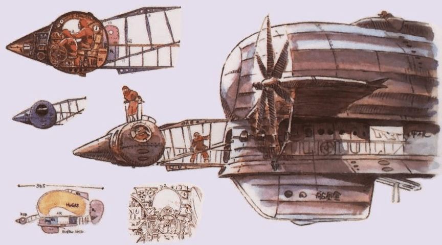
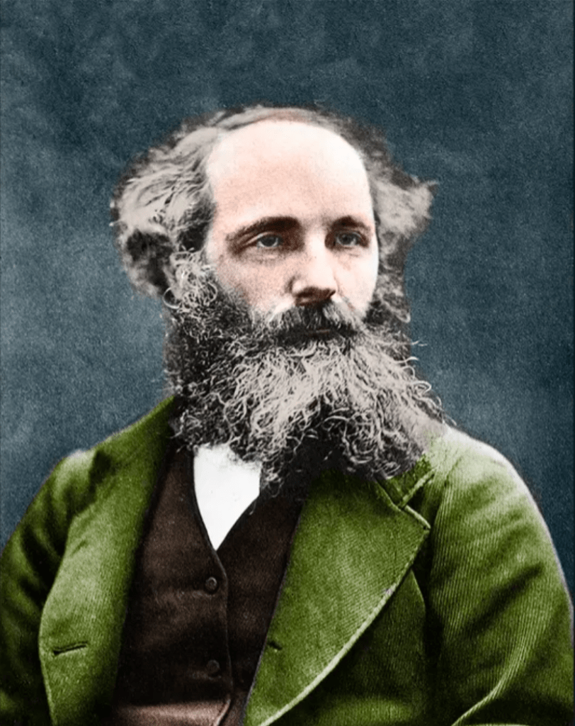
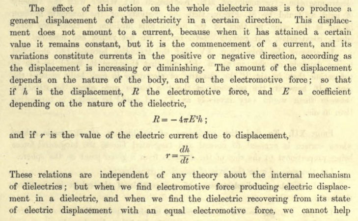
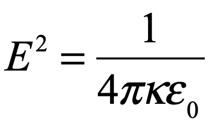
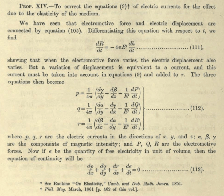
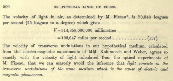
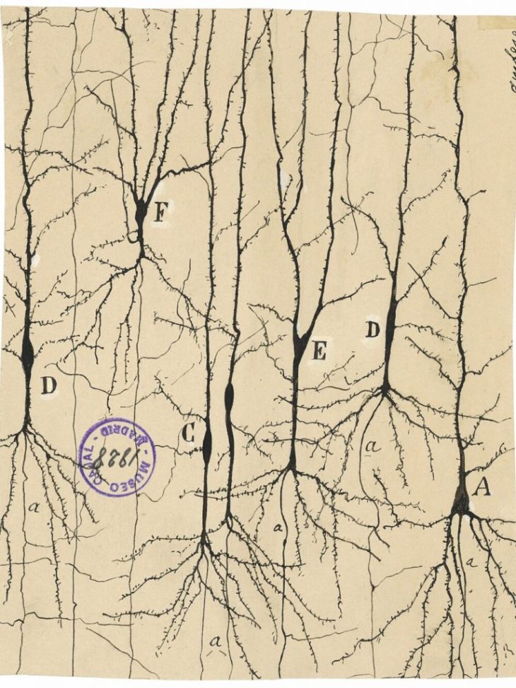
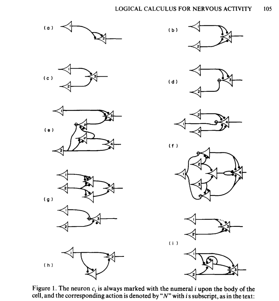
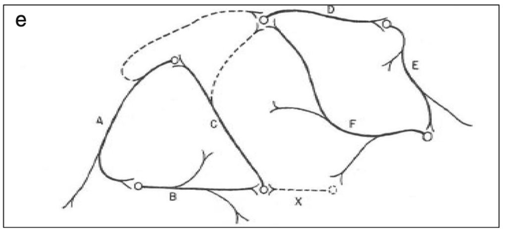
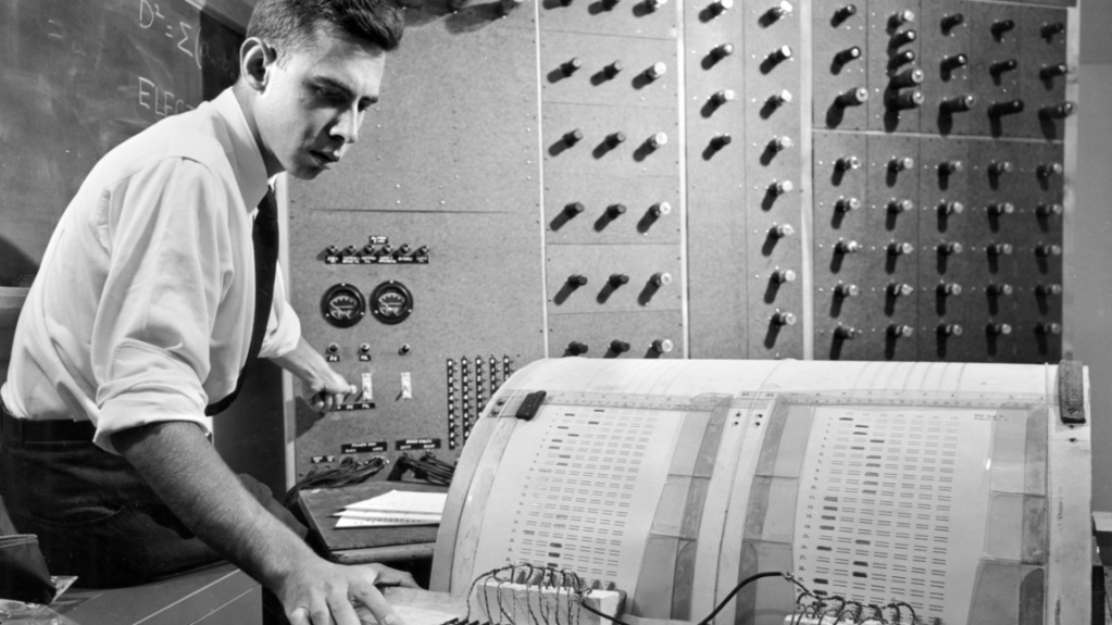
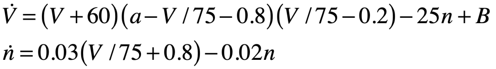
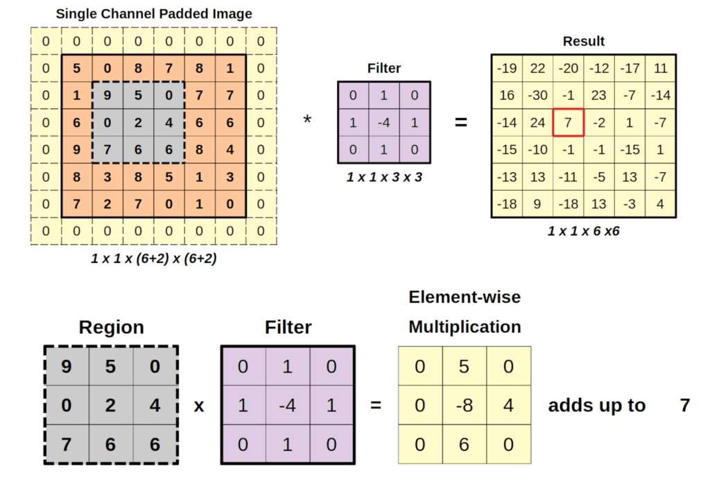
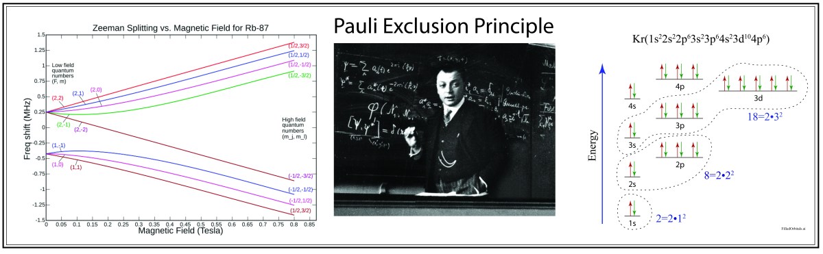
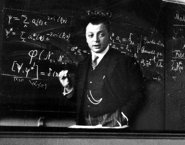
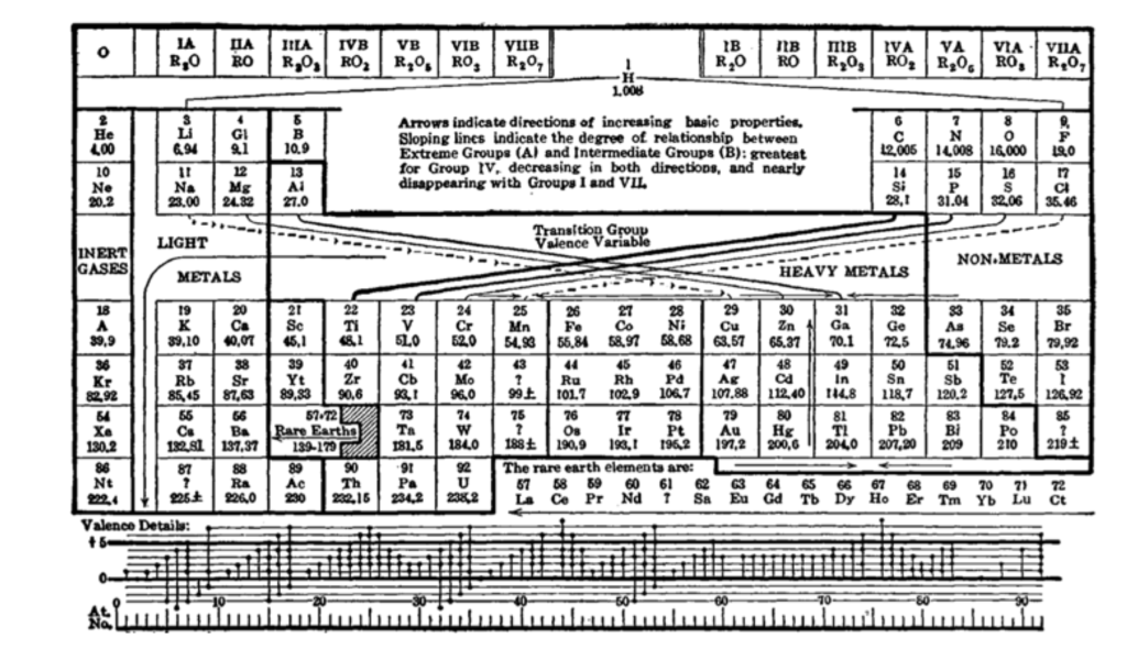
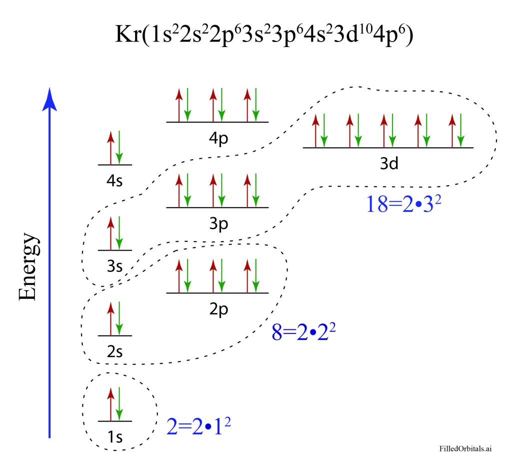
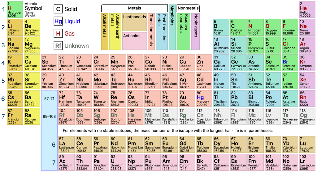
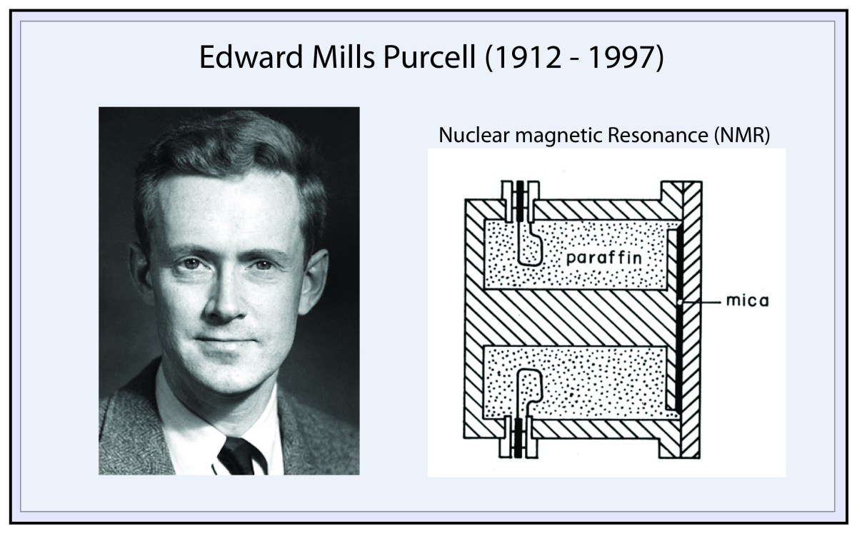
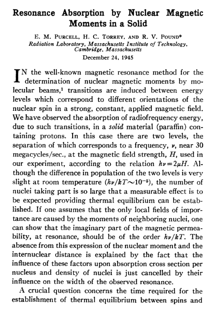
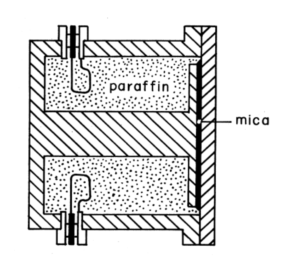
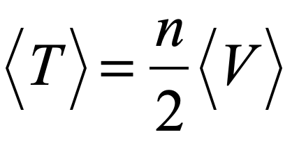
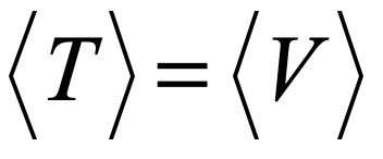
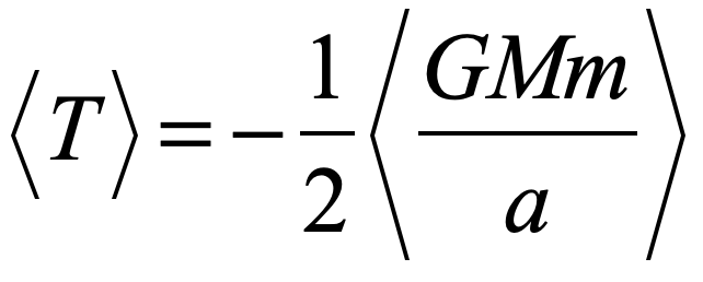
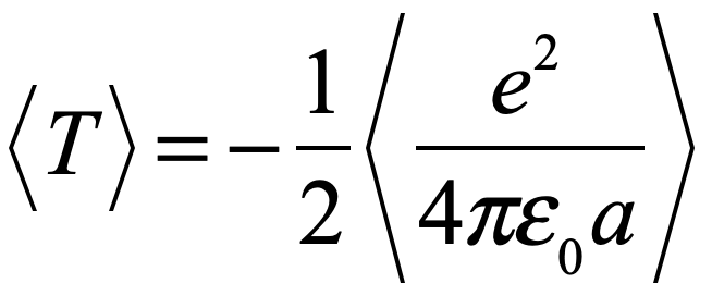
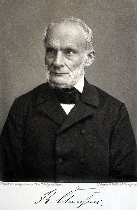
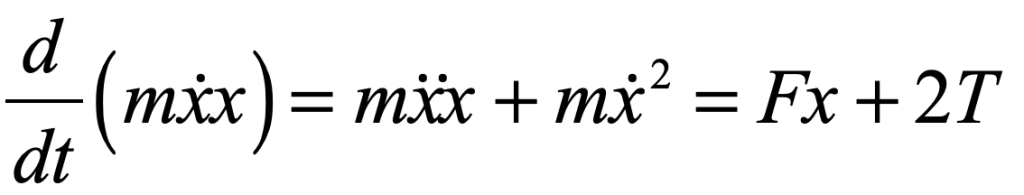
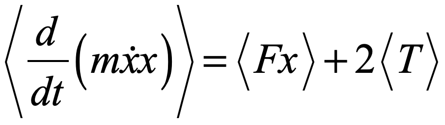
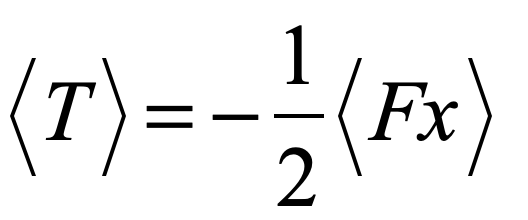
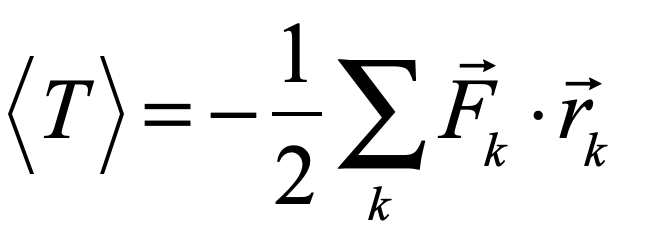
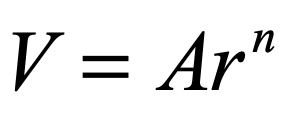
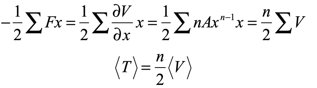
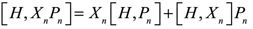
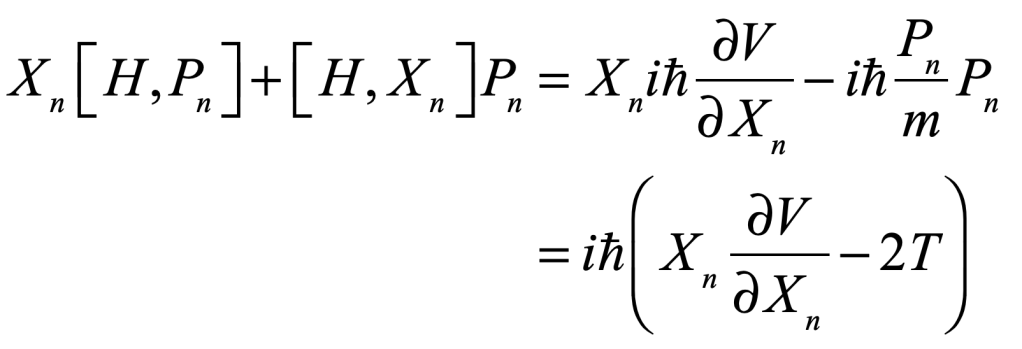
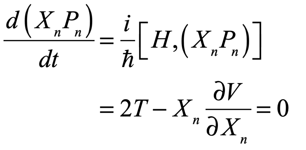
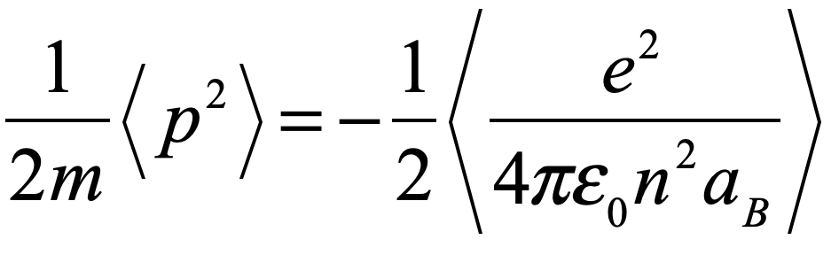
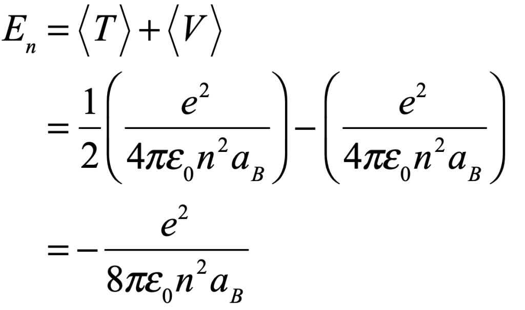
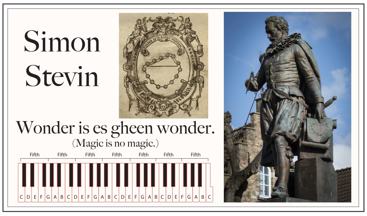
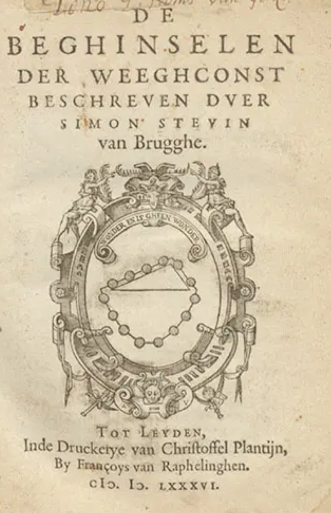
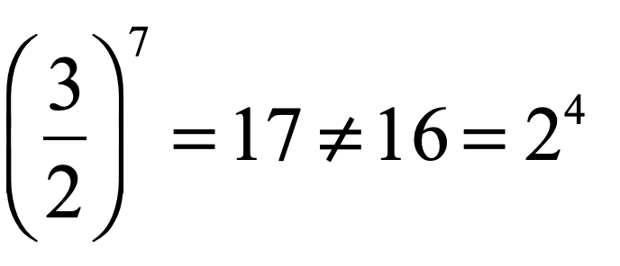
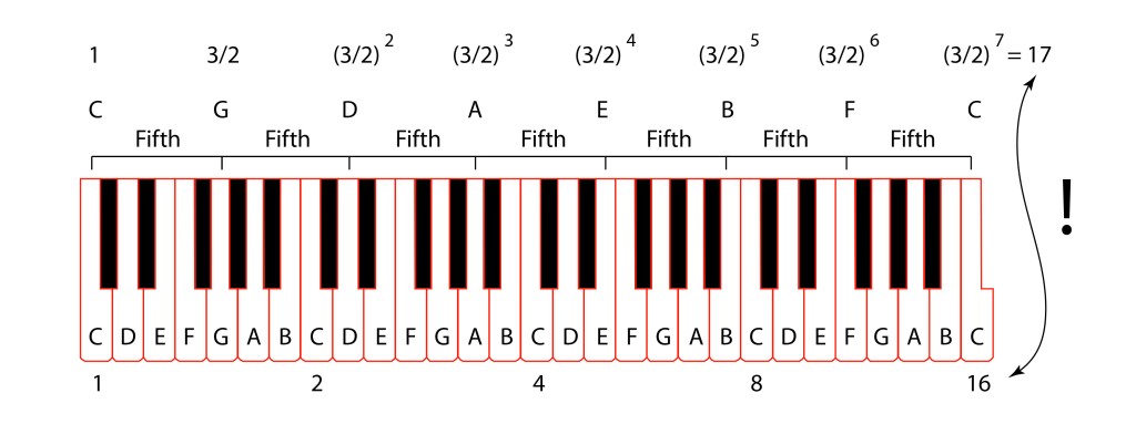
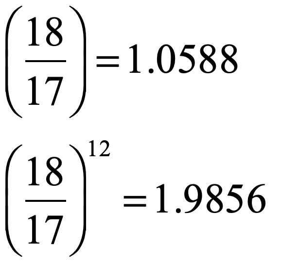
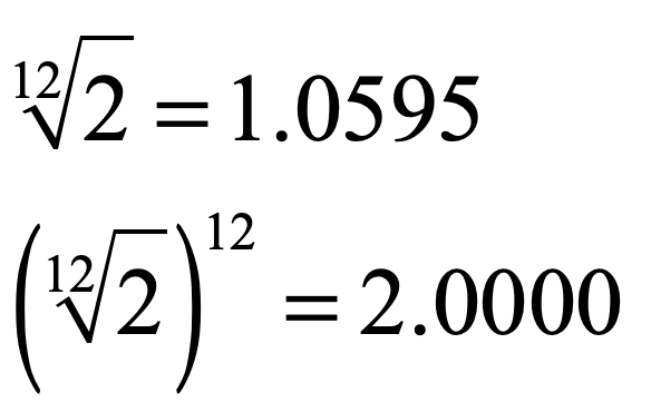
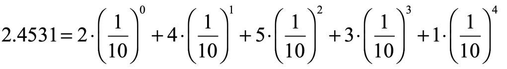
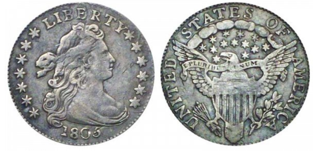
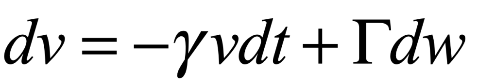
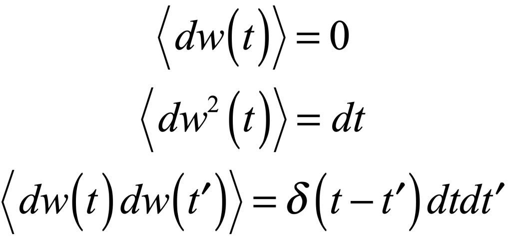
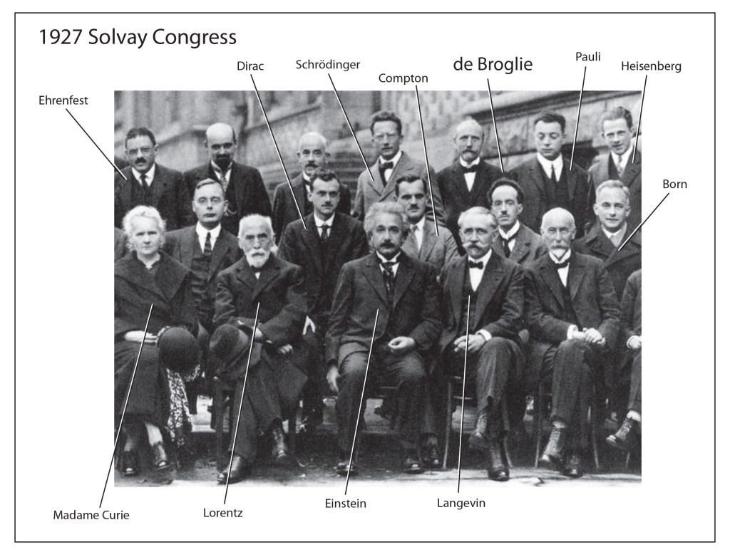
By David D. Nolte, Feb. 14, 2024

[1] L. de Broglie, “A tentative theory of light quanta,” Philosophical Magazine 47, 446-458 (1924).

January 24, 2024 by David D. Nolte

Frontiers of Physics: The Year in Review (2023)

These days, the physics breakthroughs in the news that really catch the eye tend to be Astro-centric. Partly, this is due to the new data coming from the James Webb Space Telescope, which is the flashiest and newest toy of the year in physics. But also, this is part of a broader trend in physics that we see in the interest statements of physics students applying to graduate school. With the Higgs business winding down for high energy physics, and solid state physics becoming more engineering, the frontiers of physics have pushed to the skies, where there seem to be endless surprises.

To be sure, quantum information physics (a hot topic) and AMO (atomic and molecular optics) are performing herculean feats in the laboratories. But even there, Bose-Einstein condensates are simulating the early universe, and quantum computers are simulating worm holes—tipping their hat to astrophysics!

So here are my picks for the top physics breakthroughs of 2023.

The Early Universe

The James Webb Space Telescope (JWST) has come through big on all of its promises! They said it would revolutionize the astrophysics of the early universe, and they were right. As of 2023, all astrophysics textbooks describing the early universe and the formation of galaxies are now obsolete, thanks to JWST.

Foremost among the discoveries is how fast the universe took up its current form. Galaxies condensed much earlier than expected, as did supermassive black holes. Everything that we thought took billions of years seem to have happened in only about one-tenth of that time (incredibly fast on cosmic time scales). The new JWST observations blow away the status quo on the early universe, and now the astrophysicists have to go back to the chalk board.

Fig. The JWST artist’s rendering. Image credit.

Gravitational Ripples

If LIGO and the first detection of gravitational waves was the huge breakthrough of 2015, detecting something so faint that it took a century to build an apparatus sensitive enough to detect them, then the newest observations of gravitational waves using galactic ripples presents a whole new level of gravitational wave physics.

*Fig. Ripples in spacetime.* *Image* credit.

By using the exquisitely precise timing of distant pulsars, astrophysicists have been able to detect a din of gravitational waves washing back and forth across the universe. These waves came from supermassive black hole mergers in the early universe. As the waves stretch and compress the space between us and distant pulsars, the arrival times of pulsar pulses detected at the Earth vary a tiny but measurable amount, haralding the passing of a gravitational wave.

This approach is a form of statistical optics in contrast to the original direct detection that was a form of interferometry. These are complimentary techniques in optics research, just as they will be complimentary forms of gravitational wave astronomy. Statistical optics (and fluctuation analysis) provides spectral density functions which can yield ensemble averages in the large N limit. This can answer questions about large ensembles that single interferometric detection cannot contribute to. Conversely, interferometric detection provides the details of individual events in ways that statistical optics cannot do. The two complimentary techniques, moving forward, will provide a much clearer picture of gravitational wave physics and the conditions in the universe that generate them.

Phosphorous on Enceladus

Planetary science is the close cousin to the more distant field of cosmology, but being close to home also makes it more immediate. The search for life outside the Earth stands as one of the greatest scientific quests of our day. We are almost certainly not alone in the universe, and life may be as close as Enceladus, the icy moon of Saturn.

Scientists have been studying data from the Cassini spacecraft that observed Saturn close-up for over a decade from 2004 to 2017. Enceladus has a subsurface liquid ocean that generates plumes of tiny ice crystals that erupt like geysers from fissures in the solid surface. The ocean remains liquid because of internal tidal heating caused by the large gravitational forces of Saturn.

*Fig. The Cassini Spacecraft. Imag*e credit.

The Cassini spacecraft flew through the plumes and analyzed their content using its Cosmic Dust Analyzer. While the ice crystals from Enceladus were already known to contain organic compounds, the science team discovered that they also contain phosphorous. This is the least abundant element within the molecules of life, but it is absolutely essential, providing the backbone chemistry of DNA as well as being a constituent of amino acids.

With this discovery, all the essential building blocks of life are known to exist on Enceladus, along with a liquid ocean that is likely to be in chemical contact with rocky minerals on the ocean floor, possibly providing the kind of environment that could promote the emergence of life on a planet other than Earth.

Simulating the Expanding Universe in a Bose-Einstein Condensate

Putting the universe under a microscope in a laboratory may have seemed a foolish dream, until a group at the University of Heidelberg did just that. It isn’t possible to make a real universe in the laboratory, but by adjusting the properties of an ultra-cold collection of atoms known as a Bose-Einstein condensate, the research group was able to create a type of local space whose internal metric has a curvature, like curved space-time. Furthermore, by controlling the inter-atomic interactions of the condensate with a magnetic field, they could cause the condensate to expand or contract, mimicking different scenarios for the evolution of our own universe. By adjusting the type of expansion that occurs, the scientists could create hypotheses about the geometry of the universe and test them experimentally, something that could never be done in our own universe. This could lead to new insights into the behavior of the early universe and the formation of its large-scale structure.

*Fig. Expansion of the Universe. Image* Credit

Quark Entanglement

This is the only breakthrough I picked that is not related to astrophysics (although even this effect may have played a role in the very early universe).

Entanglement is one of the hottest topics in physics today (although the idea is 89 years old) because of the crucial role it plays in quantum information physics. The topic was awarded the 2022 Nobel Prize in Physics which went to John Clauser, Alain Aspect and Anton Zeilinger.

Direct observations of entanglement have been mostly restricted to optics (where entangled photons are easily created and detected) or molecular and atomic physics as well as in the solid state.

But entanglement eluded high-energy physics (which is quantum matter personified) until 2023 when the Atlas Collaboration at the LHC (Large Hadron Collider) in Geneva posted a manuscript on Arxiv that reported the first observation of entanglement in the decay products of a quark.

*Fig. Thresholds for entanglement detection in decays from top quarks. Image* credit.

Quarks interact so strongly (literally through the strong force), that entangled quarks experience very rapid decoherence, and entanglement effects virtually disappear in their decay products. However, top quarks decay so rapidly, that their entanglement properties can be transferred to their decay products, producing measurable effects in the downstream detection. This is what the Atlas team detected.

While this discovery won’t make quantum computers any better, it does open up a new perspective on high-energy particle interactions, and may even have contributed to the properties of the primordial soup during the Big Bang.

Ramon y Cajal (1888): Visualizing Neurons

McCulloch and Pitts (1943): Mathematical Models

Donald Hebb (1949): Hebbian Learning

Hodgkin and Huxley (1952): Neuron Transporter Models

Frank Rosenblatt (1958): The Perceptron

Richard Fitzhugh and Jin-Ichi Nagumo (1961): Neural van der Pol Oscillators

John Hopfield (1982): Spin Glasses and Recurrent Networks

The Parallel Distributed Processing Group (1986): Backpropagation

Yann LeCun (1989): Convolutional Neural Networks

Geoff Hinton (2006): Deep Belief

Further Reading

References

Encyclopedia Article on Relativity

Anomalous Zeeman Effect

The Difference of Squares

The Bohr Model for Many Electrons

Pauli’s Breakthrough

Timeline:

References:

Early Days

Purdue University and Prof. Lark-Horowitz

Radiation Laboratory, MIT

Nuclear Magnetic Resonance

References and Notes

The Virial Theorem

Rudolph Clausius and his Virial Theorem

The Virial in Astrophysics

The Virial in Quantum Physics

References

Matlab Code

Early Days of the Photon

The Quantum Derivation by Bose

Enter Einstein

References

The Renaissance Man

The Law of Fall

Musical Temperament

Decimal Notation

References

Electron Spin

5-Dimensional Quantum Mechanics

Brownian Motion

Quantum Tunneling

Master Equation

Selected Works by George Uhlenbeck:

Notes:

Henri Poincare (1889)

Cartwight and Littlewood (1945)

Andrey Kolmogorov (1954)

Edward Lorenz (1963)

V. I. Arnold (1964)

Sephen Smale (1967)

Ruelle and Takens (1971)

Feigenbaum (1978)

Gleick (1987)

References

de Broglie’s Early Days

de Broglie’s Massive Photons

de Broglie’s Matter Wave

The Early Universe

Gravitational Ripples

Phosphorous on Enceladus

Simulating the Expanding Universe in a Bose-Einstein Condensate

Quark Entanglement