
Gravity bends light!
Of all the audacious proposals made by Einstein, and there were many, this one takes the cake because it should be impossible.
There can be no force of gravity on light because light has no mass. Without mass, there is no gravitational “interaction”. We all know Newton’s Law of gravity … it was one of the first equations of physics we ever learned
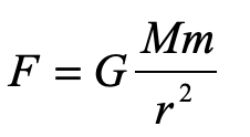
which shows the interaction between the masses M and m through their product. For light, this is strictly zero.
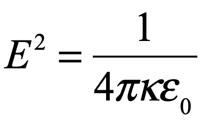
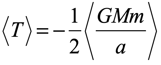
How, then did Einstein conclude, in 1907, only two years after he proposed his theory of special relativity, that gravity bends light? If it were us, we might take Newton’s other famous equation and equate the two
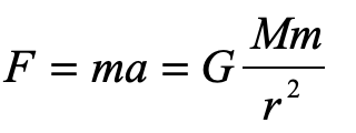
and guess that somehow the little mass m (though it equals zero) cancels out to give
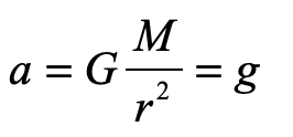
so that light would fall in gravity with the same acceleration as anything else, massive or not.
But this is not how Einstein arrived at his proposal, because this derivation is wrong! To do it right, you have to think like an Einstein.
“My Happiest Thought”
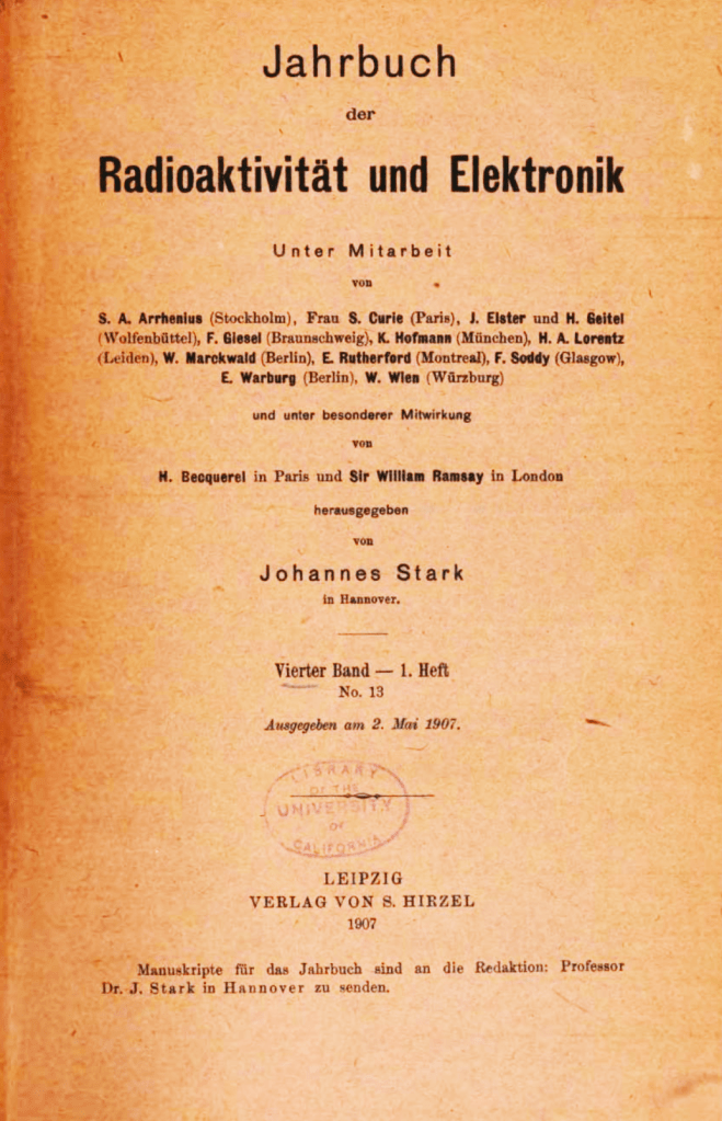
Towards the end of 1907, Einstein was asked by Johannes Stark to contribute a review article on the state of the relativity theory to the Jahrbuch of Radioactivity and Electronics. There had been a flurry of activity in the field in the two years since Einstein had published his groundbreaking paper in Annalen der Physik in September of 1905 [1]. Einstein himself had written several additional papers on the topic, along with others, so Stark felt it was time to put things into perspective.
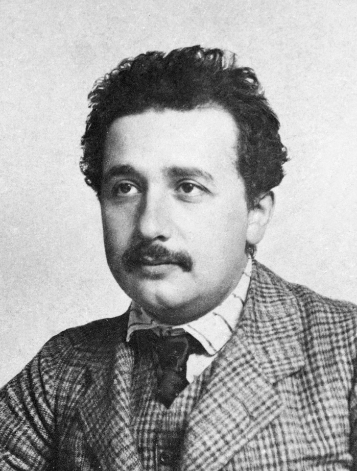
Einstein was still working at the Patent Office in Bern, Switzerland, which must not have been too taxing, because it gave him plenty of time think. It was while he was sitting in his armchair in his office in 1907 that he had what he later described as the happiest thought of his life. He had been struggling with the details of how to apply relativity theory to accelerating reference frames, a topic that is fraught with conceptual traps, when he had a flash of simplifying idea:
“Then there occurred to me the ‘glucklichste Gedanke meines Lebens,’ the happiest thought of my life, in the following form. The gravitational field has only a relative existence in a way similar to the electric field generated by magnetoelectric induction. Because for an observer falling freely from the roof of a house there exists —at least in his immediate surroundings— no gravitational field. Indeed, if the observer drops some bodies then these remain relative to him in a state of rest or of uniform motion… The observer therefore has the right to interpret his state as ‘at rest.'”[2]
In other words, the freely falling observer believes he is in an inertial frame rather than an accelerating one, and by the principle of relativity, this means that all the laws of physics in the accelerating frame must be the same as for an inertial frame. Hence, his great insight was that there must be complete equivalence between a mechanically accelerating frame and a gravitational field. This is the very first conception of his Equivalence Principle.
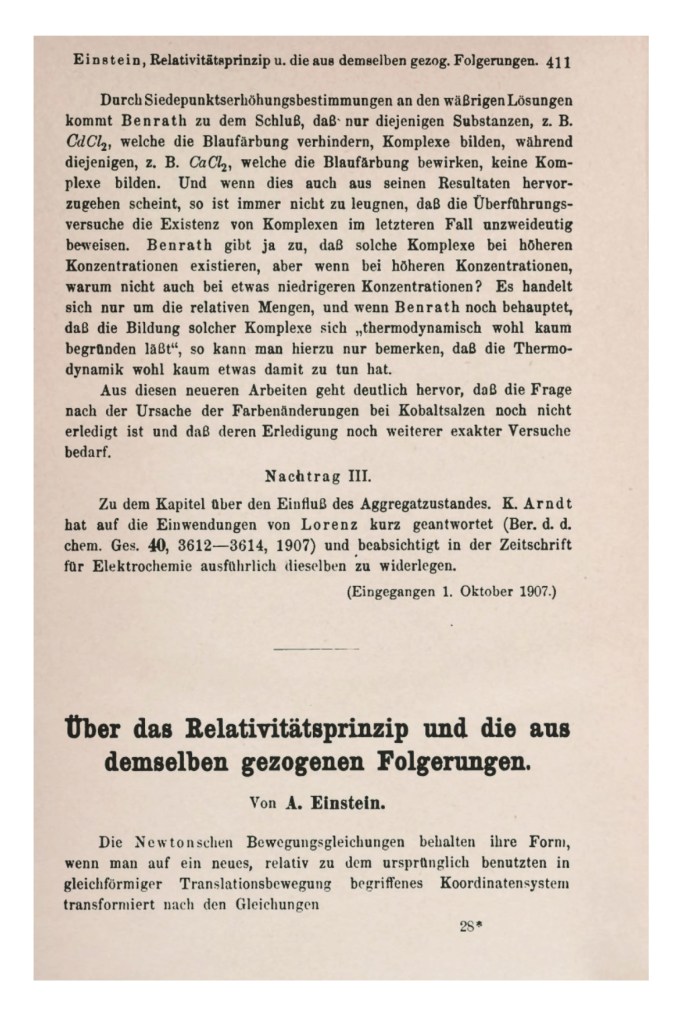
After completing his review of the consequences of special relativity in his Jahrbuch article, Einstein took the opportunity to launch into his speculations on the role of the relativity principle in gravitation. He is almost appologetic at the start, saying that:
“This is not the place for a detailed discussion of this question. But as it will occur to anybody who has been following the applications of the principle of relativity, I will not refrain from taking a stand on this question here.”
But he then launches into his first foray into general relativity with keen insights.
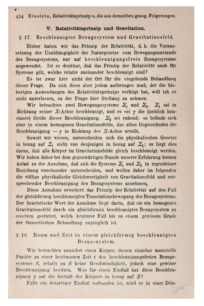
He states early in his exposition:
“… in the discussion that follows, we shall therefore assume the complete physical equivalence of a gravitational field and a corresponding accelerated reference system.”
Here is his equivalence principle. And using it, in 1907, he derives the effect of acceleration (and gravity) on ticking clocks, on the energy density of electromagnetic radiation (photons) in a gravitational potential, and on the deflection of light by gravity.
Over the next several years, Einstein was distracted by other things, such as obtaining his first university position, and his continuing work on the early quantum theory. But by 1910 he was ready to tackle the general theory of relativity once again, when he discovered that his equivalence principle was missing a key element: the effects of spatial curvature, which launched him on a 5-year program into the world of tensors and metric spaces that culminated with his completed general theory of relativity that he published in November of 1915 [4].
The Observer in the Chest: There is no Elevator
Einstein was never a stone to gather moss. Shortly after delivering his triumphal exposition on the General Theory of Relativity, he wrote up a popular account of his Special and now General Theories to be published as a book in 1916, first in German [5] and then in English [6]. What passed for a “popular exposition” in 1916 is far from what is considered popular today. Einstein’s little book is full of equations that would be somewhat challenging even for specialists. But the book also showcases Einstein’s special talent to create simple analogies, like the falling observer, that can make difficult concepts of physics appear crystal clear.
In 1916, Einstein was not yet thinking in terms of an elevator. His mental image at this time, for a sequestered observer, was someone inside a spacious chest filled with measurement apparatus that the observer could use at will. This observer in his chest was either floating off in space far from any gravitating bodies, or the chest was being pulled by a rope hooked to the ceiling such that the chest accelerates constantly. Based on the measurement he makes, he cannot distinguish between gravitational fields and acceleration, and hence they are equivalent. A bit later in the book, Einstein describes what a ray of light would do in an accelerating frame, but he does not have his observer attempt any such measurement, even in principle, because the deflection of the ray of light from a linear path would be far too small to measure.
But Einstein does go on to say that any curvature of the path of the light ray requires that the speed of light changes with position. This is a shocking admission, because his fundamental postulate of relativity from 1905 was the invariance of the speed of light in all inertial frames. It was from this simple assertion that he was eventually able to derive E = mc2. Where, on the one hand, he was ready to posit the invariance of the speed of light, on the other hand, as soon as he understood the effects of gravity on light, Einstein did not hesitate to cast this postulate adrift.
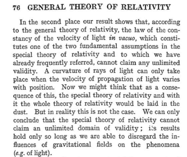
Fig. 5 Einstein’s argument for the speed of light depending on position in a gravitational field.
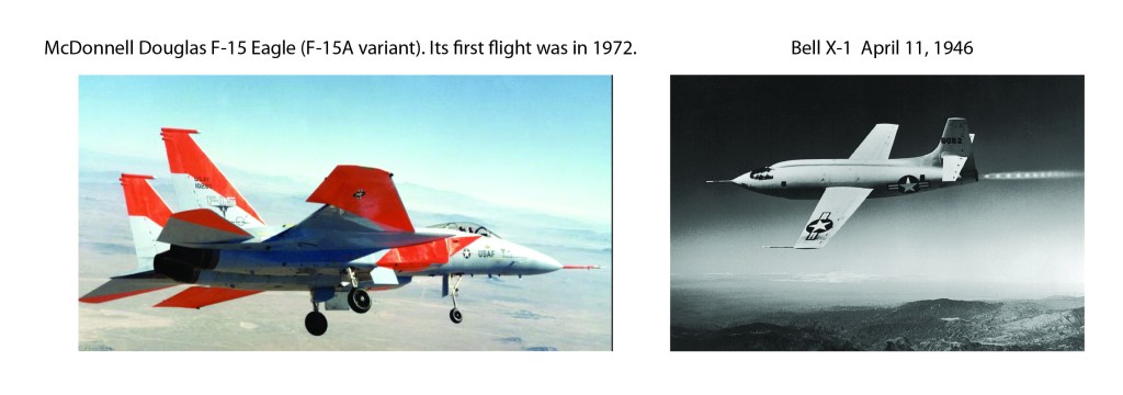
(Einstein can be forgiven for taking so long to speak in terms of an elevator that could accelerate at a rate of one g, because it was not until 1946 that the rocket plane Bell X-1 achieved linear acceleration exceeding 1 g, and jet planes did not achieve 1 g linear acceleration until the F-15 Eagle in 1972.)
The Evolution of Physics: Enter Einstein’s Elevator
Years passed, and Einstein fled an increasingly autocratic and belligerent Germany for a position at Princeton’s Institute for Advanced Study. In 1938, at the instigation of his friend Leopold Infeld, they decided to write a general interest book on the new physics of relativity and quanta that had evolved so rapidly over the past 30 years.
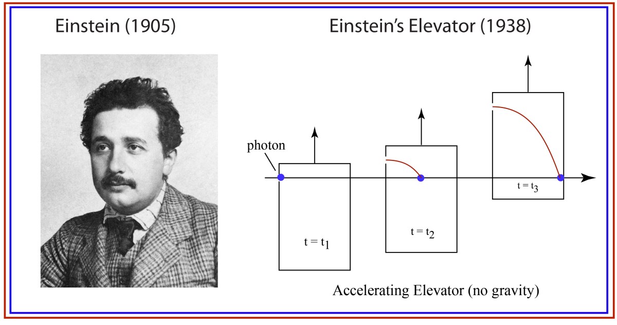
Here, in this obscure book that no-one remembers today, we find Einstein’s elevator for the first time, and the exposition talks very explicitly about a small window that lets in a light ray, and what the observer sees (in principle) for the path of the ray.
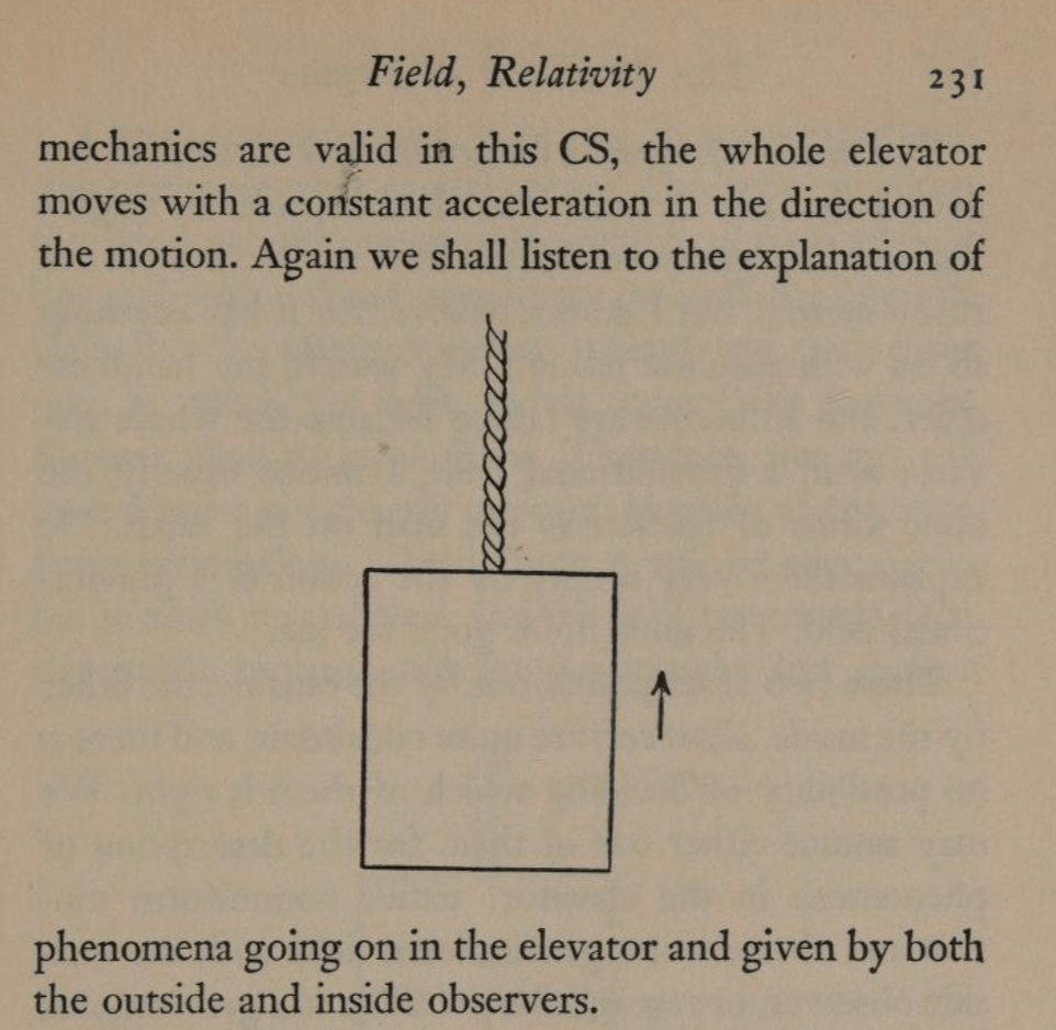
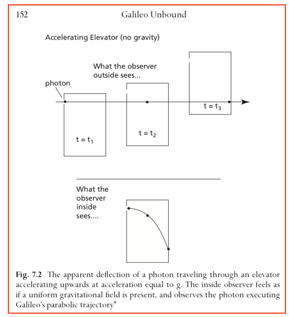
By the equivalence principle, the observer cannot tell whether they are far out in space, being accelerated at the rate g, or whether they are statinary on the surface of the Earth subject to a gravitational field. In the first instance of the accelerating elevator, a photon moving in a straight line through space would appear to deflect downward in the elevator, as shown in Fig. 9, because the elevator is accelerating upwards as the photon transits the elevator. However, by the equivalence principle, the same physics should occur in the gravitational field. Hence, gravity must bend light. Furthermore, light falls inside the elevator with an acceleration g, just as any other object would.
Light Deflection in the Equivalence Principle
A photon enters an elevator at right angles to its acceleration vector g. Use the geodesic equation and the elevator (Equivalence Principle) metric [8]
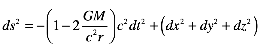
to show that the trajectory is parabolic. (This is a classic HW problem from Introduction to Modern Dynamics.)
Solution:
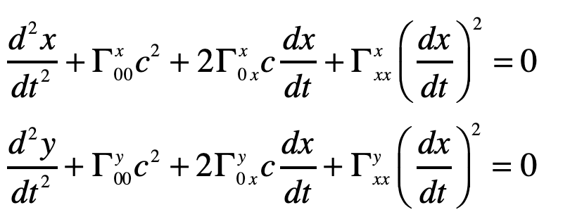
The geodesic equation with time as the dependent variable
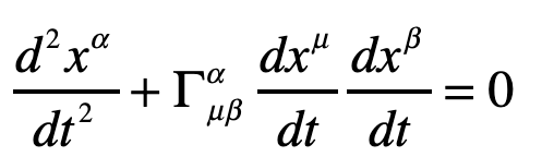
This gives two coordinate equations
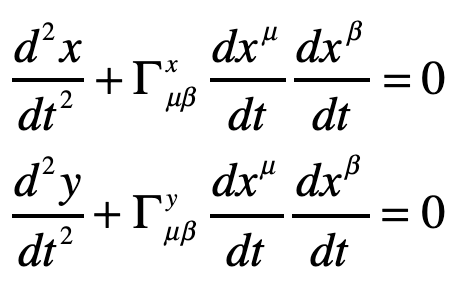
Note that x0 = ct and x1 = ct are both large relative to the y-motion of the photon. The metric component that is relevant here is
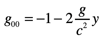
and the others are unity. The geodesic becomes (assuming dy/dt = 0)
The Christoffel symbols are
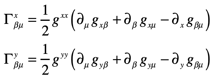
which give
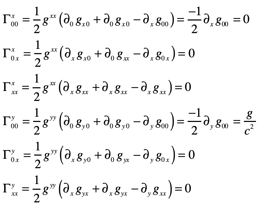
Therefore
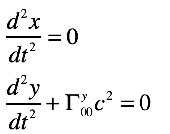
or
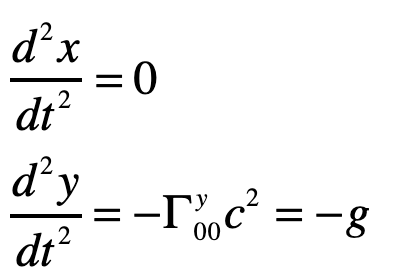
where the photon falls with acceleration g, as anticipated.
Light Deflection in the Schwarzschild Metric
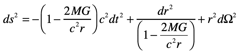
Do the same problem of the light ray in Einstein’s Elevator, but now using the full Schwarzschild solution to the Einstein Field equations.
Solution:
Einstein’s elevator is the classic test of virtually all heuristic questions related to the deflection of light by gravity. In the previous Example, the deflection was attributed to the Equivalence Principal in which the observer in the elevator cannot discern whether they are in an acceleration rocket ship or standing stationary on Earth. In that case, the time-like metric component is the sole cause of the free-fall of light in gravity. In the Schwarzschild metric, on the other hand, the curvature of the field near a spherical gravitating body also contributes. In this case, the geodesic equation, assuming that dr/dt = 0 for the incoming photon, is
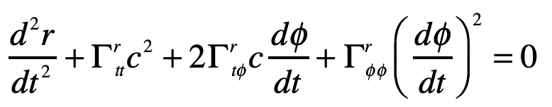
where, as before, the Christoffel symbol for the radial displacements are
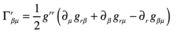
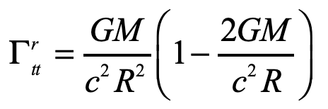
Evaluating one of these

The other Christoffel symbol that contributes to the radial motion is
and the geodesic equation becomes
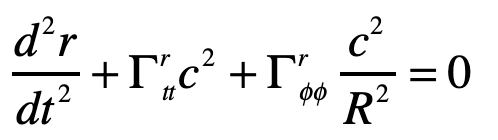
with
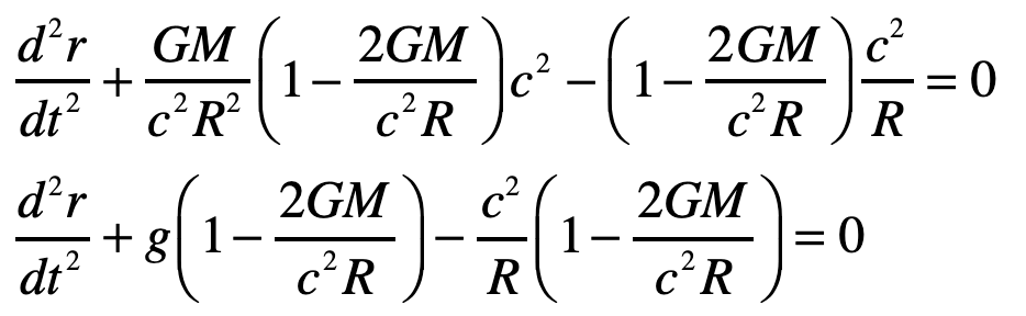
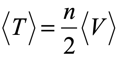
The radial acceleration of the light ray in the elevator is thus
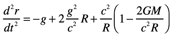
The first term on right is free-fall in gravity, just as was obtained from the Equivalence Principal. The second term is a higher-order correction caused by curvature of spacetime. The third term is the motion of the light ray relative to the curved ceiling of the elevator in this spherical geometry and hence is a kinematic (or geometric) artefact. (It is interesting that the GR correction on the curved-ceiling correction is of the same order as the free-fall term, so one would need to be very careful doing such an experiment … if it were at all measurable.) Therefore, the second and third terms are curved-geometry effects while the first term is the free fall of the light ray.
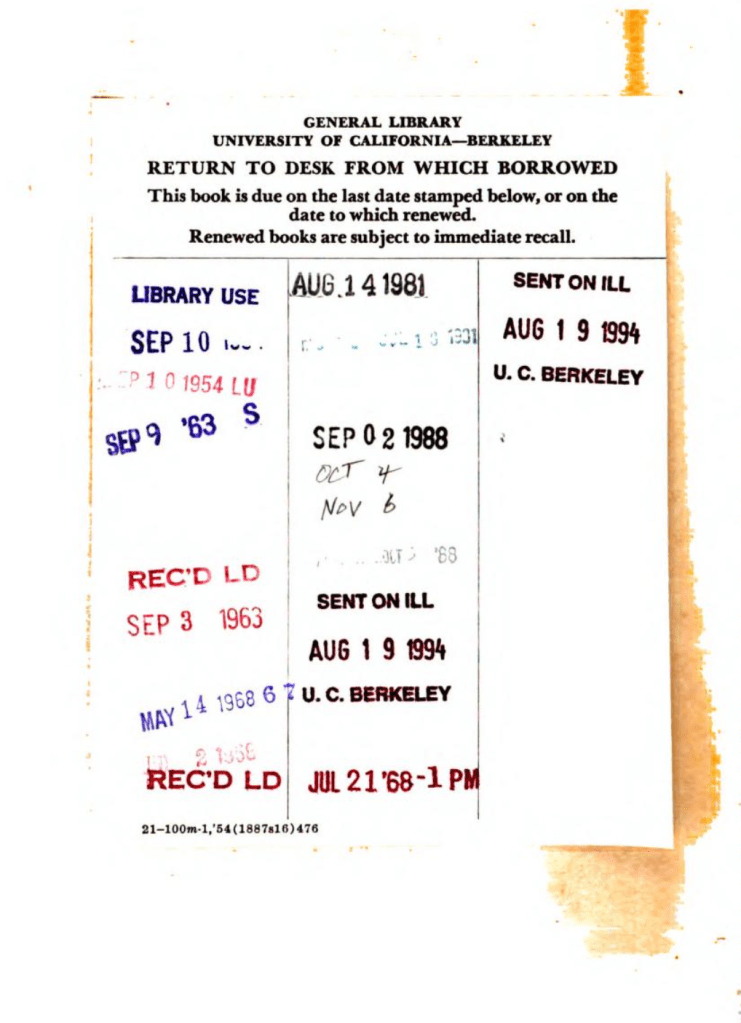
Post-Script: The Importance of Library Collections
I was amused to see the library card of the scanned Internet Archive version of Einstein’s Jahrbuch article, shown below. The volume was checked out in August of 1981 from the UC Berkeley Physics Library. It was checked out again 7 years later in September of 1988. These dates coincide with when I arrived at Berkeley to start grad school in physics, and when I graduated from Berkeley to start my post-doc position at Bell Labs. Hence this library card serves as the book ends to my time in Berkeley, a truly exhilarating place that was the top-ranked physics department at that time, with 7 active Nobel Prize winners on its faculty.
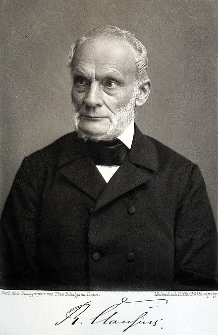
During my years at Berkeley, I scoured the stacks of the Physics Library looking for books and journals of historical importance, and was amazed to find the original volumes of Annalen der Physik from 1905 where Einstein published his famous works. This was the same library where, ten years before me, John Clauser was browsing the stacks and found the obscure paper by John Bell on his inequalities that led to Clauser’s experiment on entanglement that won him the Nobel Prize of 2022.
That library at UC Berkeley was recently closed, as was the Physics Library in my department at Purdue University (see my recent Blog), where I also scoured the stacks for rare gems. Some ancient books that I used to be able to check out on a whim, just to soak up their vintage ambience and to get a tactile feel for the real thing held in my hands, are now not even available through Interlibrary Loan. I may be able to get scans from Internet Archive online, but the palpable magic of the moment of discovery is lost.
References:
[1] Einstein, A. (1905). Zur Elektrodynamik bewegter Körper. Annalen der Physik, 17(10), 891–921.
[2] Pais, A (2005). Subtle is the Lord: The Science and Life of Albert Einstein (Oxford University Press). pg. 178
[3] Einstein, A. (1907). Über das Relativitätsprinzip und die aus demselben gezogenen Folgerungen. Jahrbuch der Radioaktivität und Elektronik, 4, 411–462.
[4] A. Einstein (1915), “On the general theory of relativity,” Sitzungsberichte Der Koniglich Preussischen Akademie Der Wissenschaften, pp. 778-786, Nov.
[5] Einstein, A. (1916). Über die spezielle und die allgemeine Relativitätstheorie (Gemeinverständlich). Braunschweig: Friedr. Vieweg & Sohn.
[6] Einstein, A. (1920). Relativity: The Special and the General Theory (A Popular Exposition) (R. W. Lawson, Trans.). London: Methuen & Co. Ltd.
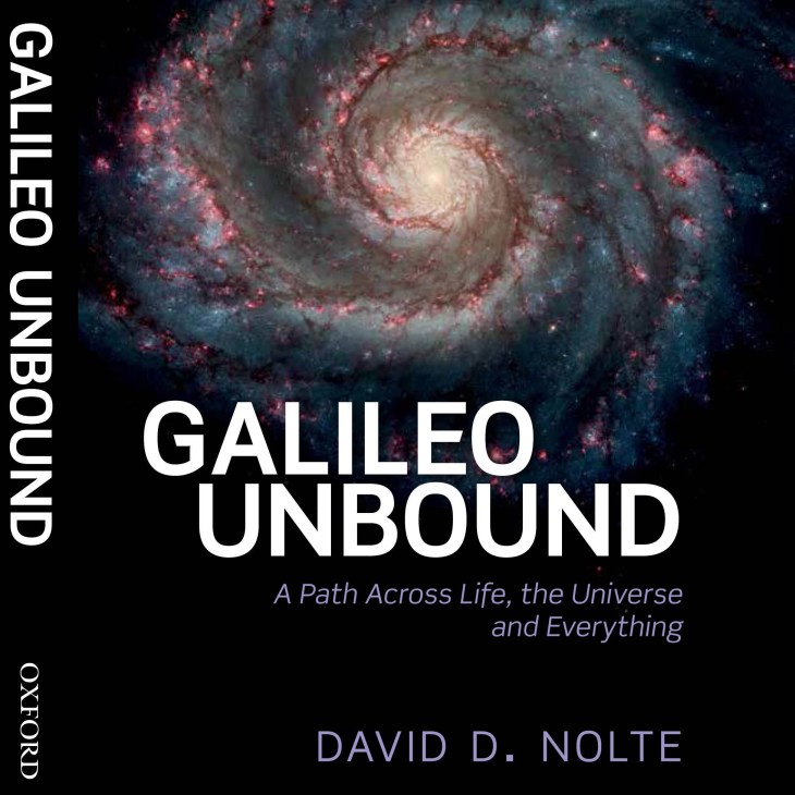
[7] Nolte, D. D. (2018). Galileo Unbound. A Path Across Life, the Universe and Everything. (Oxford University Press)
[8] Nolte, D. D. (2019). Introduction to Modern Dynamics: Chaos, Networks, Space and Time (Oxford University Press).


.jpg)