Physicists of the nineteenth century were obsessed with mechanical models. They must have dreamed, in their sleep, of spinning flywheels connected by criss-crossing drive belts turning enmeshed gears. For them, Newton’s clockwork universe was more than a metaphor—they believed that mechanical description of a phenomenon could unlock further secrets and act as a tool of discovery.
It is no wonder they thought this way—the mid-eighteenth century was at the peak of the industrial revolution, dominated by the steam engine and the profusion of mechanical power and gears across broad swaths of society.
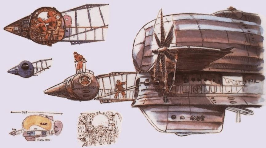
Steampunk
The Victorian obsession with steam and power is captured beautifully in the literary and animé genre known as Steampunk. The genre is alternative historical fiction that portrays steam technology progressing into grand and wild new forms as electrical and gasoline technology fail to develop. An early classic in the genre is Miyazaki’s 1986 anime´ film Castle in the Sky (1986) by Hayao Miyazaki about a world where all mechanical devices, including airships, are driven by steam. A later archetype of the genre is the 2004 animé film Steam Boy (2004) by Katsuhiro Otomo about the discovery of superwater that generates unlimited steam power. As international powers vie to possess it, mad scientists strive to exploit it for society, but they create a terrible weapon instead. One of the classics that helped launch the genre is the novel The Difference Engine (1990) by William Gibson and Bruce Sterling that envisioned an alternative history of computers developed by Charles Babbage and Ada Lovelace.
Steampunk is an apt, if excessively exaggerated, caricature of the Victorian mindset and approach to science. Confidence in microscopic mechanical models among natural philosophers was encouraged by the success of molecular models of ideal gases as the foundation for macroscopic thermodynamics. Pictures of small perfect spheres colliding with each other in simple billiard-ball-like interactions could be used to build up to overarching concepts like heat and entropy and temperature. Kinetic theory was proposed in 1857 by the German physicist Rudolph Clausius and was quickly placed on a firm physical foundation using principles of Hamiltonian dynamics by the British physicist James Clerk Maxwell.
James Clerk Maxwell
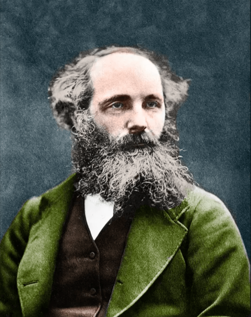
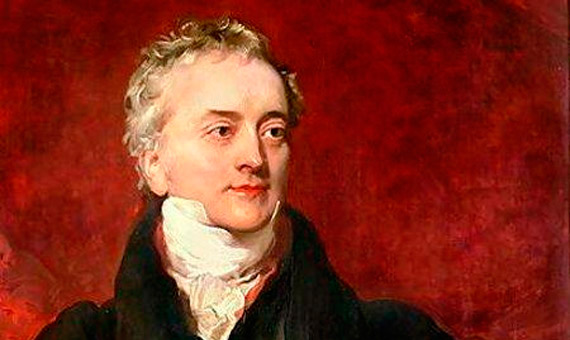
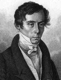
James Clerk Maxwell (1831 – 1879) was one of three titans out of Cambridge who served as the intellectual leaders in mid-nineteenth-century Britain. The two others were George Stokes and William Thomson (Lord Kelvin). All three were Wranglers, the top finishers on the Tripos exam at Cambridge, the grueling eight-day examination across all fields of mathematics. The winner of the Tripos, known as first Wrangler, was announced with great fanfare in the local papers, and the lucky student was acclaimed like a sports hero is today. Stokes in 1841 was first Wrangler while Thomson (Lord Kelvin) in 1845 and Maxwell in 1854 were each second Wranglers. They were also each winners of the Smith’s Prize, the top examination at Cambridge for mathematical originality. When Maxwell sat for the Smith’s Prize in 1854 one of the exam problems was a proof written by Stokes on a suggestion by Thomson. Maxwell failed to achieve the proof, though he did win the Prize. The problem became known as Stokes’ Theorem, one of the fundamental theorems of vector calculus, and the proof was eventually provided by Hermann Hankel in 1861.
After graduation from Cambridge, Maxwell took the chair of natural philosophy at Marischal College in the city of Aberdeen in Scotland. He was only 25 years old when he began, fifteen years younger than any of the other professors. He split his time between the university and his family home at Glenlair in the south of Scotland, which he inherited from his father the same year he began his chair at Aberdeen. His research interests spanned from the perception of color to the rings of Saturn. He improved on Thomas Young’s three-color theory by correctly identifying red, green and blue as the primary receptors of the eye and invented a scheme for adding colors that is close to the HSV (hue-saturation-value) system used today in computer graphics. In his work on the rings of Saturn, he developed a statistical mechanical approach to explain how the large-scale structure emerged from the interactions among the small grains. He applied these same techniques several years later to the problem of ideal gases when he derived the speed distribution known today as the Maxwell-Boltzmann distribution.
Maxwell’s career at Aberdeen held great promise until he was suddenly fired from his post in 1860 when Marischal College merged with nearby King’s College to form the University of Aberdeen. After the merger, the university had the abundance of two professors of Natural Philosophy while needing only one, and Maxwell was the junior. With his new wife, Maxwell retired to Glenlair and buried himself in writing the first drafts of a paper titled “On Physical Lines of Force” [2]. The paper explored the mathematical and mechanical aspects of the curious lines of magnetic force that Michael Faraday had first proposed in 1831 and which Thomson had developed mathematically around 1845 as the first field theory in physics.
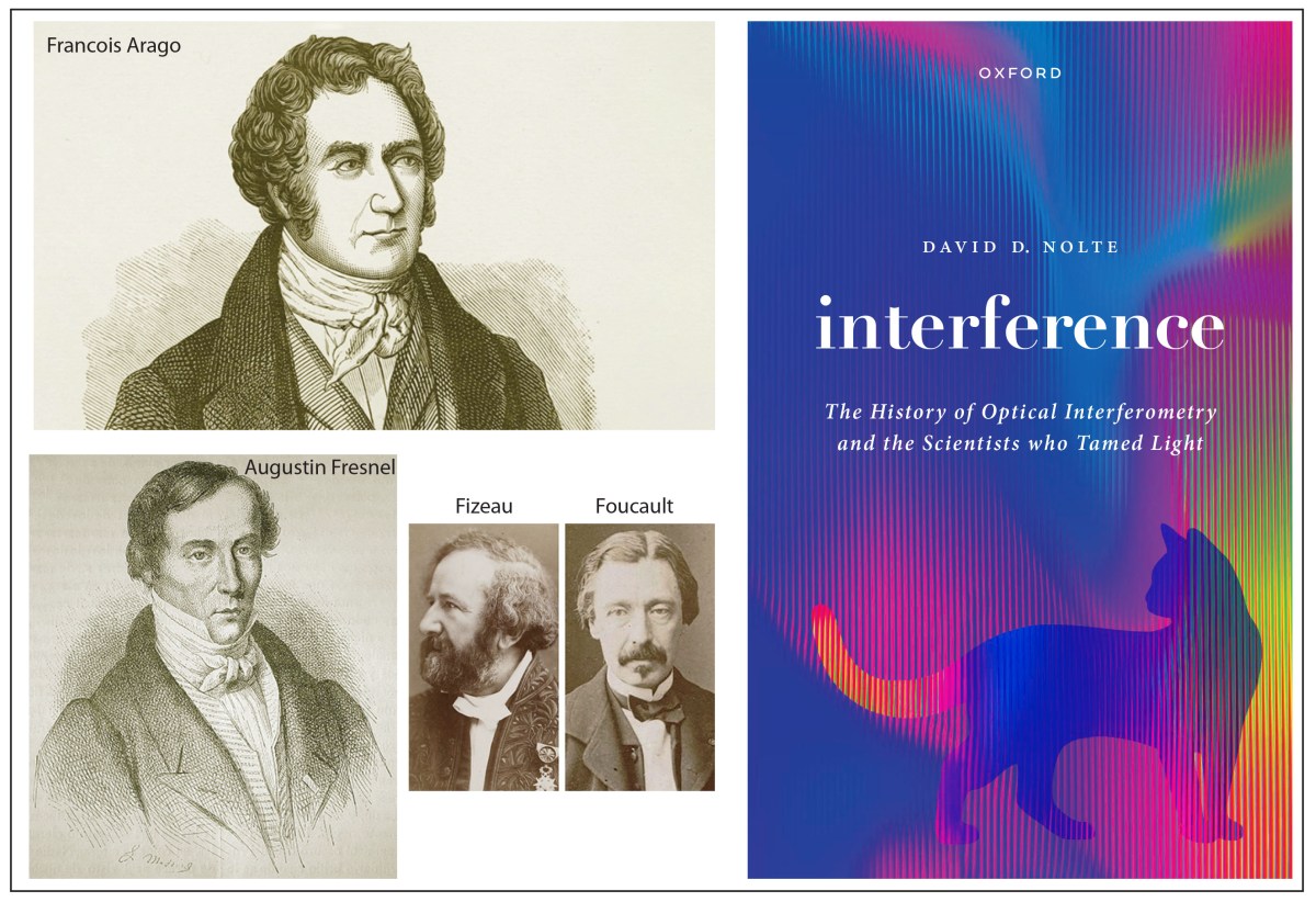
As Maxwell explored the interrelationships among electric and magnetic phenomena, he derived a wave equation for the electric and magnetic fields and was astounded to find that the speed of electromagnetic waves was essentially the same as the speed of light. The importance of this coincidence did not escape him, and he concluded that light—that rarified, enigmatic and quintessential fifth element—must be electromagnetic in origin. Ever since Francois Arago and Agustin Fresnel had shown that light was a wave phenomenon, scientists had been searching for other physical signs of the medium that supported the waves—a medium known as the luminiferous aether (or ether). With Maxwell’s new finding, it meant that the luminiferous ether must be related to electric and magnetic fields. In the Steampunk tradition of his day, Maxwell began a search for a mechanical model. He did not need to look far, because his friend Thomson had already built a theory on a foundation provided by the Irish mathematician James MacCullagh (1809 – 1847)
The Luminiferous Ether
The late 1830’s was a busy time for the luminiferous ether. Agustin-Louis Cauchy published his extensive theory of the ether in 1836, and the self-taught George Green published his highly influential mathematical theory in 1838 which contained many new ideas, such as the emphasis on potentials and his derivation of what came to be called Green’s theorem.
In 1839 MacCullagh took an approach that established a core property of the ether that later inspired both Thomson and Maxwell in their development of electromagnetic field theory. What McCullagh realized was that the energy of the ether could be considered as if it had both kinetic energy and potential energy (ideas and nomenclature that would come several decades later). Most insightful was the fact that the potential energy of the field depended on pure rotation like a vortex. This rotationally elastic ether was a mathematical invention without any mechanical analog, but it successfully described reflection and refraction as well as polarization of light in crystalline optics.
In 1856 Thomson put Faraday’s famous magneto-optic rotation of light (the Faraday Effect discovered by Faraday in 1845) into mathematical form and began putting Faraday’s initially abstract ideas of the theory of fields into concrete equations. He drew from MacCullagh’s rotational ether as well as an idea from William Rankine about the molecular vortex model of atoms to develop a mechanical vortex model of the ether. Thomson explained how the magnetic field rotated the linear polarization of light through the action of a multiplicity of molecular vortices. Inspired by Thomson, Maxwell took up the idea of molecular vortices as well as Faraday’s magnetic induction in free space and transferred the vortices from being a property exclusively of matter to being a property of the luminiferous ether that supported the electric and magnetic fields.
Maxwellian Cogwheels
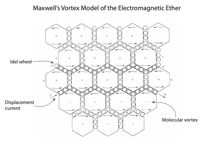
Maxwell’s model of the electromagnetic fields in the ether is the apex of Victorian mechanistic philosophy—too explicit to be a true model of reality—yet it was amazingly fruitful as a tool of discovery, helping Maxwell develop his theory of electrodynamics. The model consisted of an array of elastic vortex cells separated by layers of small particles that acted as “idle wheels” to transfer spin from one vortex to another . The magnetic field was represented by the rotation of the vortices, and the electric current was represented by the displacement of the idle wheels.
Fig. 1 Maxwell’s vortex model of the electromagnetic ether. The molecular vortices rotate according to the direction of the magnetic field, supported by idle wheels. The physical displacement of the idle wheels became an analogy for Maxwell’s displacement current [2].
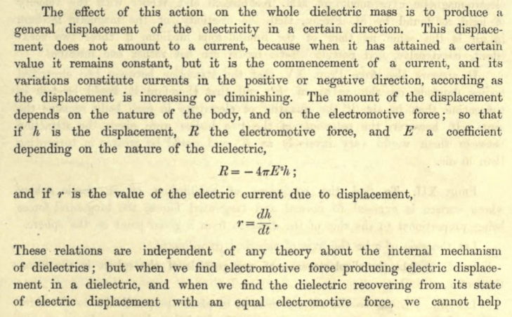
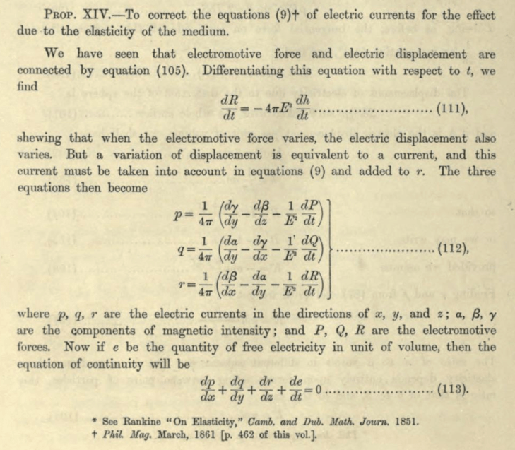
Two predictions by this outrightly mechanical model were to change the physics of electromagnetism forever: First, any change in strain in the electric field would cause the idle wheels to shift, creating a transient current that was called a “displacement current”. This displacement current was one of the last pieces in the electromagnetic puzzle that became Maxwell’s equations.
Fig. 2 In “Physical Lines of Force” in 1861, Maxwell introduces the idea of a displacement current [RefLink].
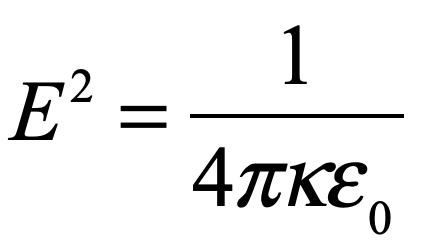
In this description, E is not the electric field, but is related to the dielectric permativity through the relation
Maxwell went further to prove his Proposition XIV on the contribution of the displacement current to conventional electric currents.
Fig. 3 Maxwell’s Proposition XIV on adding the displacement current to the conventional electric current [RefLink].
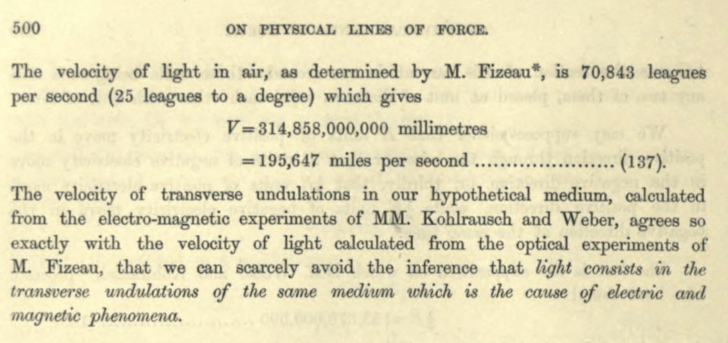
Second, Maxwell calculated that this elastic vortex ether propagated waves at a speed that was close to the known speed of light measured a decade previously by the French physicist Hippolyte Fizeau. He remarked, “we can scarcely avoid the inference that light consists of the transverse undulations of the same medium which is the cause of electric and magnetic phenomena.” [1] This was the first direct prediction that light, previously viewed as a physical process separate from electric and magnetic fields, was an electromagnetic phenomenon.
Fig. 4 Maxwell’s calculation of the speed of light in his mechanical ether. It matched closely the measured speed of light [RefLink].
These two predictions—of the displacement current and the electromagnetic origin of light—have stood the test of time and are center pieces of Maxwells’s legacy. How strange that they arose from a mechanical model of vortices and idle wheels like so many cogs and gears in the machinery powering the Victorian age, yet such is the power of physical visualization.
[1] pg. 12, The Maxwellians, Bruce Hunt (Cornell University Press, 1991)
[2] Maxwell, J. C. (1861). “On physical lines of force”. Philosophical Magazine. 90: 11–23.
Light is one of the most powerful manifestations of the forces of physics because it tells us about our reality. The interference of light, in particular, has led to the detection of exoplanets orbiting distant stars, discovery of the first gravitational waves, capture of images of black holes and much more. The stories behind the history of light and interference go to the heart of how scientists do what they do and what they often have to overcome to do it. These time-lines are organized along the chapter titles of the book Interference. They follow the path of theories of light from the first wave-particle debate, through the personal firestorms of Albert Michelson, to the discoveries of the present day in quantum information sciences.
Thomas Young was the ultimate dabbler, his interests and explorations ranged far and wide, from ancient egyptology to naval engineering, from physiology of perception to the physics of sound and light. Yet unlike most dabblers who accomplish little, he made original and seminal contributions to all these fields. Some have called him the “Last Man Who Knew Everything“.
Thomas Young. The Law of Interference.
Topics: The Law of Interference. The Rosetta Stone. Benjamin Thompson, Count Rumford. Royal Society. Christiaan Huygens. Pendulum Clocks. Icelandic Spar. Huygens’ Principle. Stellar Aberration. Speed of Light. Double-slit Experiment.
1629 – Huygens born (1629 – 1695)
1642 – Galileo dies, Newton born (1642 – 1727)
1655 – Huygens ring of Saturn
1657 – Huygens patents the pendulum clock
1666 – Newton prismatic colors
1666 – Huygens moves to Paris
1669 – Bartholin double refraction in Icelandic spar
1670 – Bartholinus polarization of light by crystals
1671 – Expedition to Hven by Picard and Rømer
1673 – James Gregory bird-feather diffraction grating
1801 – Young Theory of Light and Colours, three color mechanism (Bakerian Lecture), Young considers interference to cause the colored films, first estimates of the wavelengths of different colors
1802 – Young begins series of lecturs at the Royal Institution (Jan. 1802 – July 1803)
1802 – Young names the principle (Law) of interference
Augustin Fresnel was an intuitive genius whose talents were almost squandered on his job building roads and bridges in the backwaters of France until he was discovered and rescued by Francois Arago.
Topics: Particles versus Waves. Malus and Polarization. Agustin Fresnel. Francois Arago. Diffraction. Daniel Bernoulli. The Principle of Superposition. Joseph Fourier. Transverse Light Waves.
1665 – Grimaldi diffraction bands outside shadow
1673 – James Gregory bird-feather diffraction grating
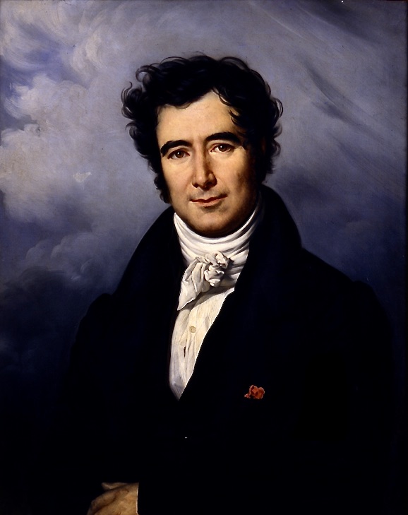
There is no question that Francois Arago was a swashbuckler. His life’s story reads like an adventure novel as he went from being marooned in hostile lands early in his career to becoming prime minister of France after the 1848 revolutions swept across Europe.
Topics: The Birth of Interferometry. Snell’s Law. Fresnel and Arago. The First Interferometer. Fizeau and Foucault. The Speed of Light. Ether Drag. Jamin Interferometer.
No name is more closely connected to interferometry than that of Albert Michelson. He succeeded, sometimes at great personal cost, in launching interferometric metrology as one of the most important tools used by scientists today.
Albert A. Michelson, 1907 Nobel Prize. Image Credit.
Topics: The Trials of Albert Michelson. Hermann von Helmholtz. Michelson and Morley. Fabry and Perot.
1810 – Arago search for ether drag
1813 – Fraunhofer dark lines in Sun spectrum
1813 – Faraday begins at Royal Institution
1820 – Oersted discovers electromagnetism
1821 – Faraday electromagnetic phenomena
1827 – Green mathematical analysis of electricity and magnetism
1830 – Cauchy ether as elastic solid
1831 – Faraday electromagnetic induction
1831 – Cauchy ether drag
1831 – Maxwell born
1831 – Faraday electromagnetic induction
1836 – Cauchy’s second theory of the ether
1838 – Green theory of the ether
1839 – Hamilton group velocity
1839 – MacCullagh properties of rotational ether
1839 – Cauchy ether with negative compressibility
1841 – Maxwell entered Edinburgh Academy (age 10) met P. G. Tait
1842 – Doppler effect
1845 – Faraday effect (magneto-optic rotation)
1846 – Stokes’ viscoelastic theory of the ether
1847 – Maxwell entered Edinburgh University
1850 – Maxwell at Cambridge, studied under Hopkins, also knew Stokes and Whewell
1852 – Michelson born Strelno, Prussia
1854 – Maxwell wins the Smith’s Prize (Stokes’ theorem was one of the problems)
1855 – Michelson’s immigrate to San Francisco through Panama Canal
Learning from his attempts to measure the speed of light through the ether, Michelson realized that the partial coherence of light from astronomical sources could be used to measure their sizes. His first measurements using the Michelson Stellar Interferometer launched a major subfield of astronomy that is one of the most active today.
R Hanbury Brown
Topics: Measuring the Stars. Astrometry. Moons of Jupiter. Schwarzschild. Betelgeuse. Michelson Stellar Interferometer. Banbury Brown Twiss. Sirius. Adaptive Optics.
1838 – Bessel stellar parallax measurement with Fraunhofer telescope
1868 – Fizeau proposes stellar interferometry
1873 – Stephan implements Fizeau’s stellar interferometer on Sirius, sees fringes
1880 – Michelson Idea for second-order measurement of relative motion against ether
1880 – 1882 Michelson Studies in Europe (Helmholtz in Berlin, Quincke in Heidelberg, Cornu, Mascart and Lippman in Paris)
1881 – Michelson Measurement at Potsdam with funds from Alexander Graham Bell
1881 – Michelson Resigned from active duty in the Navy
1883 – Michelson Joined Case School of Applied Science
1889 – Michelson moved to Clark University at Worcester
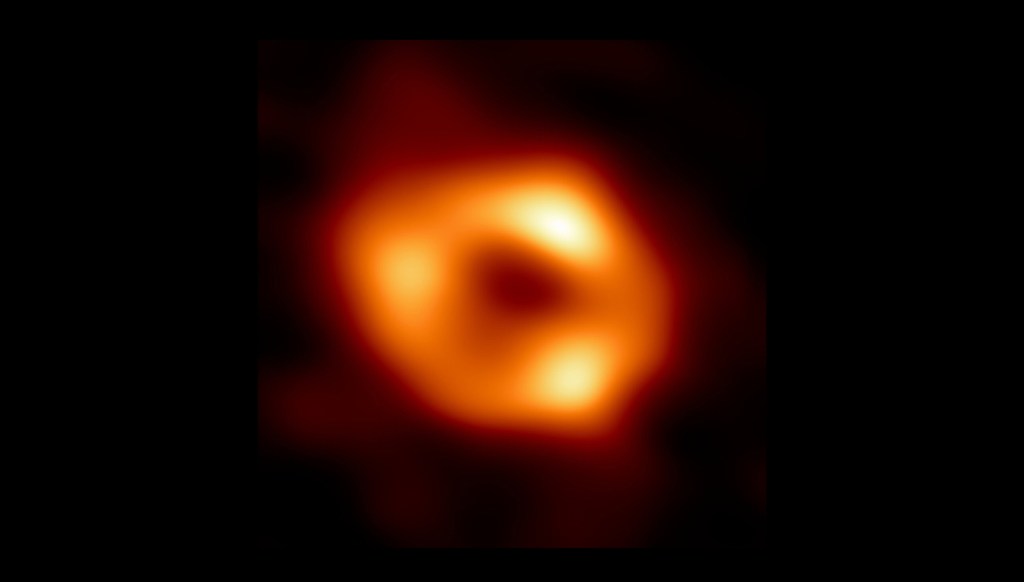
Stellar interferometry is opening new vistas of astronomy, exploring the wildest occupants of our universe, from colliding black holes half-way across the universe (LIGO) to images of neighboring black holes (EHT) to exoplanets near Earth that may harbor life.
Image of the supermassive black hole in M87 from Event Horizon Telescope.
Topics: Gravitational Waves, Black Holes and the Search for Exoplanets. Nulling Interferometer. Event Horizon Telescope. M87 Black Hole. Long Baseline Interferometry. LIGO.
1947 – Virgo A radio source identified as M87
1953 – Horace W. Babcock proposes adaptive optics (AO)
From the astronomically large dimensions of outer space to the microscopically small dimensions of inner space, optical interference pushes the resolution limits of imaging.
Topics: Diffraction and Interference. Joseph Fraunhofer. Diffraction Gratings. Henry Rowland. Carl Zeiss. Ernst Abbe. Phase-contrast Microscopy. Super-resolution Micrscopes. Structured Illumination.
The coherence of laser light is like a brilliant jewel that sparkles in the darkness, illuminating life, probing science and projecting holograms in virtual worlds.
What is the image of one photon interfering? Better yet, what is the image of two photons interfering? The answer to this crucial question laid the foundation for quantum communication.
Topics: The Beginnings of Quantum Communication. EPR paradox. Entanglement. David Bohm. John Bell. The Bell Inequalities. Leonard Mandel. Single-photon Interferometry. HOM Interferometer. Two-photon Fringes. Quantum cryptography. Quantum Teleportation.
1900 – Planck (1901). “Law of energy distribution in normal spectra.” [1]
There is almost no technical advantage better than having exponential resources at hand. The exponential resources of quantum interference provide that advantage to quantum computing which is poised to usher in a new era of quantum information science and technology.
David Deutsch.
Topics: Interferometric Computing. David Deutsch. Quantum Algorithm. Peter Shor. Prime Factorization. Quantum Logic Gates. Linear Optical Quantum Computing. Boson Sampling. Quantum Computational Advantage.
1980 – Paul Benioff describes possibility of quantum computer
[10] B. R. Mollow, R. J. Glauber: Phys. Rev. 160, 1097 (1967); 162, 1256 (1967)
[11] J. F. Clauser, M. A. Horne, A. Shimony, and R. A. Holt, ” Proposed experiment to test local hidden-variable theories,” Physical Review Letters, vol. 23, no. 15, pp. 880-&, (1969)
[15] R. Ghosh and L. Mandel, “Observation of nonclassical effects in the interference of 2 photons,” Physical Review Letters, vol. 59, no. 17, pp. 1903-1905, Oct (1987)
[16] C. K. Hong, Z. Y. Ou, and L. Mandel, “Measurement of subpicosecond time intervals between 2 photons by interference,” Physical Review Letters, vol. 59, no. 18, pp. 2044-2046, Nov (1987)
[18] D. Deutsch, “QUANTUM-THEORY, THE CHURCH-TURING PRINCIPLE AND THE UNIVERSAL QUANTUM COMPUTER,” Proceedings of the Royal Society of London Series a-Mathematical Physical and Engineering Sciences, vol. 400, no. 1818, pp. 97-117, (1985)
[19] P. W. Shor, “ALGORITHMS FOR QUANTUM COMPUTATION – DISCRETE LOGARITHMS AND FACTORING,” in 35th Annual Symposium on Foundations of Computer Science, Proceedings, S. Goldwasser Ed., (Annual Symposium on Foundations of Computer Science, 1994, pp. 124-134.
[20] F. Arute et al., “Quantum supremacy using a programmable superconducting processor,” Nature, vol. 574, no. 7779, pp. 505-+, Oct 24 (2019)
[21] H.-S. Zhong et al., “Quantum computational advantage using photons,” Science, vol. 370, no. 6523, p. 1460, (2020)
Further Reading: The History of Light and Interference (2023)
This history of interferometry has many surprising back stories surrounding the scientists who discovered and explored one of the most important aspects of the physics of light—interference. From Thomas Young who first proposed the law of interference, and Augustin Fresnel and Francois Arago who explored its properties, to Albert Michelson, who went almost mad grappling with literal firestorms surrounding his work, these scientists overcame personal and professional obstacles on their quest to uncover light’s secrets. The book’s stories, told around the topic of optics, tells us something more general about human endeavor as scientists pursue science.
Interference: The History of Optical Interferometry and the Scientists who Tamed Light, was published Ag. 6 and is available at Oxford University Press and Amazon. Here is a brief preview of the frist several chapters:
Chapter 1. Thomas Young Polymath: The Law of Interference
Thomas Young was the ultimate dabbler, his interests and explorations ranged far and wide, from ancient egyptology to naval engineering, from physiology of perception to the physics of sound and light. Yet unlike most dabblers who accomplish little, he made original and seminal contributions to all these fields. Some have called him the “Last Man Who Knew Everything”.
Thomas Young. The Law of Interference.
The chapter, Thomas Young Polymath: The Law of Interference, begins with the story of the invasion of Egypt in 1798 by Napoleon Bonaparte as the unlikely link among a set of epic discoveries that launched the modern science of light. The story of interferometry passes from the Egyptian campaign and the discovery of the Rosetta Stone to Thomas Young. Young was a polymath, known for his facility with languages that helped him decipher Egyptian hieroglyphics aided by the Rosetta Stone. He was also a city doctor who advised the admiralty on the construction of ships, and he became England’s premier physicist at the beginning of the nineteenth century, building on the wave theory of Huygens, as he challenged Newton’s particles of light. But his theory of the wave nature of light was controversial, attracting sharp criticism that would pass on the task of refuting Newton to a new generation of French optical physicists.
Chapter 2. The Fresnel Connection: Particles versus Waves
Augustin Fresnel was an intuitive genius whose talents were almost squandered on his job building roads and bridges in the backwaters of France until he was discovered and rescued by Francois Arago.
The Fresnel Connection: Particles versus Waves describes the campaign of Arago and Fresnel to prove the wave nature of light based on Fresnel’s theory of interfering waves in diffraction. Although the discovery of the polarization of light by Etienne Malus posed a stark challenge to the undulationists, the application of wave interference, with the superposition principle of Daniel Bernoulli, provided the theoretical framework for the ultimate success of the wave theory. The final proof came through the dramatic demonstration of the Spot of Arago.
Chapter 3. At Light Speed: The Birth of Interferometry
There is no question that Francois Arago was a swashbuckler. His life’s story reads like an adventure novel as he went from being marooned in hostile lands early in his career to becoming prime minister of France after the 1848 revolutions swept across Europe.
At Light Speed: The Birth of Interferometry tells how Arago attempted to use Snell’s Law to measure the effect of the Earth’s motion through space but found no effect, in contradiction to predictions using Newton’s particle theory of light. Direct measurements of the speed of light were made by Hippolyte Fizeau and Leon Foucault who originally began as collaborators but had an epic falling-out that turned into an intense competition. Fizeau won priority for the first measurement, but Foucault surpassed him by using the Arago interferometer to measure the speed of light in air and water with increasing accuracy. Jules Jamin later invented one of the first interferometric instruments for use as a refractometer.
Chapter 4. After the Gold Rush: The Trials of Albert Michelson
No name is more closely connected to interferometry than that of Albert Michelson. He succeeded, sometimes at great personal cost, in launching interferometric metrology as one of the most important tools used by scientists today.
Albert A. Michelson, 1907 Nobel Prize. Image Credit.
After the Gold Rush: The Trials of Albert Michelson tells the story of Michelson’s youth growing up in the gold fields of California before he was granted an extraordinary appointment to Annapolis by President Grant. Michelson invented his interferometer while visiting Hermann von Helmholtz in Berlin, Germany, as he sought to detect the motion of the Earth through the luminiferous ether, but no motion was detected. After returning to the States and a faculty position at Case University, he met Edward Morley, and the two continued the search for the Earth’s motion, concluding definitively its absence. The Michelson interferometer launched a menagerie of interferometers (including the Fabry-Perot interferometer) that ushered in the golden age of interferometry.
Chapter 5. Stellar Interference: Measuring the Stars
Learning from his attempts to measure the speed of light through the ether, Michelson realized that the partial coherence of light from astronomical sources could be used to measure their sizes. His first measurements using the Michelson Stellar Interferometer launched a major subfield of astronomy that is one of the most active today.
R Hanbury Brown
Stellar Interference: Measuring the Stars brings the story of interferometry to the stars as Michelson proposed stellar interferometry, first demonstrated on the Galilean moons of Jupiter, followed by an application developed by Karl Schwarzschild for binary stars, and completed by Michelson with observations encouraged by George Hale on the star Betelgeuse. However, the Michelson stellar interferometry had stability limitations that were overcome by Hanbury Brown and Richard Twiss who developed intensity interferometry based on the effect of photon bunching. The ultimate resolution of telescopes was achieved after the development of adaptive optics that used interferometry to compensate for atmospheric turbulence.
And More
The last 5 chapters bring the story from Michelson’s first stellar interferometer into the present as interferometry is used today to search for exoplanets, to image distant black holes half-way across the universe and to detect gravitational waves using the most sensitive scientific measurement apparatus ever devised.
Chapter 6. Across the Universe: Exoplanets, Black Holes and Gravitational Waves
Moving beyond the measurement of star sizes, interferometry lies at the heart of some of the most dramatic recent advances in astronomy, including the detection of gravitational waves by LIGO, the imaging of distant black holes and the detection of nearby exoplanets that may one day be visited by unmanned probes sent from Earth.
Chapter 7. Two Faces of Microscopy: Diffraction and Interference
The complement of the telescope is the microscope. Interference microscopy allows invisible things to become visible and for fundamental limits on image resolution to be blown past with super-resolution at the nanoscale, revealing the intricate workings of biological systems with unprecedented detail.
Chapter 8. Holographic Dreams of Princess Leia: Crossing Beams
Holography is the direct legacy of Young’s double slit experiment, as coherent sources of light interfere to record, and then reconstruct, the direct scattered fields from illuminated objects. Holographic display technology promises to revolutionize virtual reality.
Chapter 9. Photon Interference: The Foundations of Quantum Communication and Computing
Quantum information science, at the forefront of physics and technology today, owes much of its power to the principle of interference among single photons.
Chapter 10. The Quantum Advantage: Interferometric Computing
Photonic quantum systems have the potential to usher in a new information age using interference in photonic integrated circuits.
A popular account of the trials and toils of the scientists and engineers who tamed light and used it to probe the universe.
When Galileo trained his crude telescope on the planet Jupiter, hanging above the horizon in 1610, and observed moons orbiting a planet other than Earth, it created a quake whose waves have rippled down through the centuries to today. Never had such hard evidence been found that supported the Copernican idea of non-Earth-centric orbits, freeing astronomy and cosmology from a thousand years of error that shaded how people thought.
The Earth, after all, was not the center of the Universe.
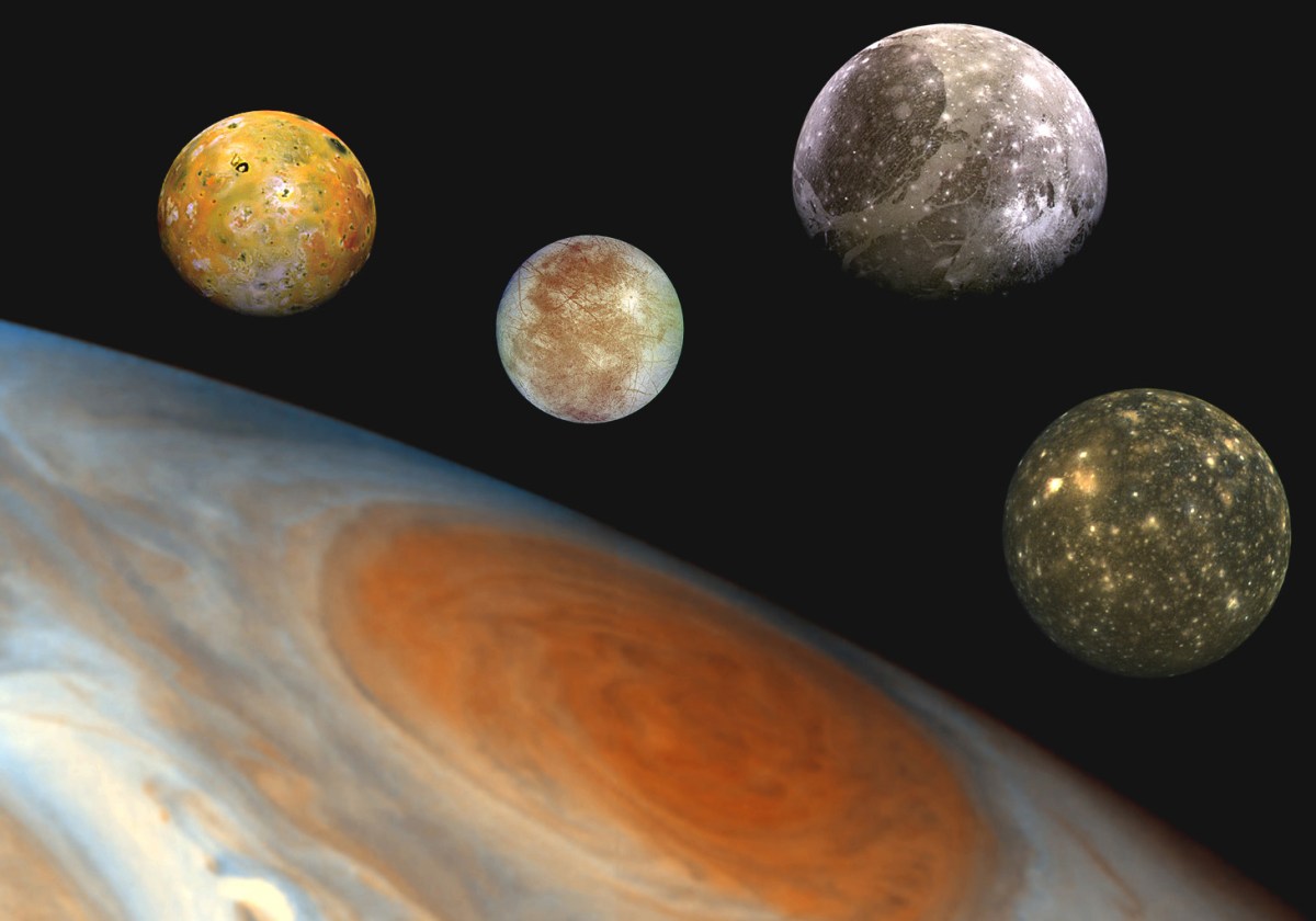
Galileo’s moons: the Galilean Moons—Io, Europa, Ganymede, and Callisto—have drawn our eyes skyward now for over 400 years. They have been the crucible for numerous scientific discoveries, serving as a test bed for new ideas and new techniques, from the problem of longitude to the speed of light, from the birth of astronomical interferometry to the beginnings of exobiology. Here is a short history of Galileo’s Moons in the history of physics.
Galileo (1610): Celestial Orbits
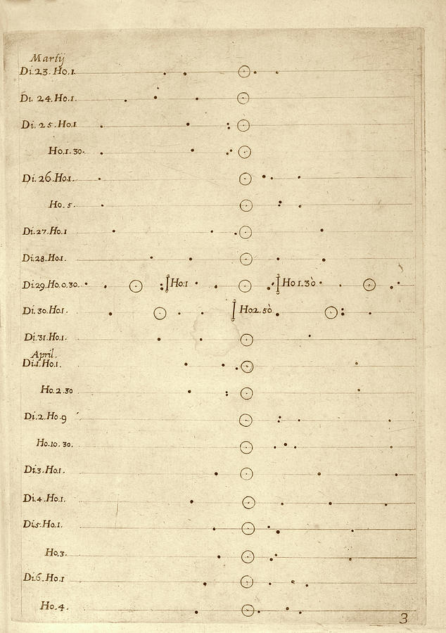
In late 1609, Galileo (1564 – 1642) received an unwelcome guest to his home in Padua—his mother. She was not happy with his mistress, and she was not happy with his chosen profession, but she was happy to tell him so. By the time she left in early January 1610, he was yearning for something to take his mind off his aggravations, and he happened to point his new 20x telescope in the direction of the planet Jupiter hanging above the horizon [1]. Jupiter appeared as a bright circular spot, but nearby were three little stars all in line with the planet. The alignment caught his attention, and when he looked again the next night, the position of the stars had shifted. On successive nights he saw them shift again, sometimes disappearing into Jupiter’s bright disk. Several days later he realized that there was a fourth little star that was also behaving the same way. At first confused, he had a flash of insight—the little stars were orbiting the planet. He quickly understood that just as the Moon orbited the Earth, these new “Medicean Planets” were orbiting Jupiter. In March 1610, Galileo published his findings in Siderius Nuncius (The Starry Messenger).
Page from Galileo’s Starry Messenger showing the positions of the moon of Jupiter
It is rare in the history of science for there not to be a dispute over priority of discovery. Therefore, by an odd chance of fate, on the same nights that Galileo was observing the moons of Jupiter with his telescope from Padua, the German astronomer Simon Marius (1573 – 1625) also was observing them through a telescope of his own from Bavaria. It took Marius four years to publish his observations, long after Galileo’s Siderius had become a “best seller”, but Marius took the opportunity to claim priority. When Galileo first learned of this, he called Marius “a poisonous reptile” and “an enemy of all mankind.” But harsh words don’t settle disputes, and the conflicting claims of both astronomers stood until the early 1900’s when a scientific enquiry looked at the hard evidence. By that same odd chance of fate that had compelled both men to look in the same direction around the same time, the first notes by Marius in his notebooks were dated to a single day after the first notes by Galileo! Galileo’s priority survived, but Marius may have had the last laugh. The eternal names of the “Galilean” moons—Io, Europe, Ganymede and Callisto—were given to them by Marius.
Picard and Cassini (1671): Longitude
The 1600’s were the Age of Commerce for the European nations who relied almost exclusively on ships and navigation. While latitude (North-South) was easily determined by measuring the highest angle of the sun above the southern horizon, longitude (East-West) relied on clocks which were notoriously inaccurate, especially at sea.
The Problem of Determining Longitude at Sea is the subject of Dava Sobel’s thrilling book Longitude (Walker, 1995) [2] where she reintroduced the world to what was once the greatest scientific problem of the day. Because almost all commerce was by ships, the determination of longitude at sea was sometimes the difference between arriving safely in port with a cargo or being shipwrecked. Galileo knew this, and later in his life he made a proposal to the King of Spain to fund a scheme to use the timings of the eclipses of his moons around Jupiter to serve as a “celestial clock” for ships at sea. Galileo’s grant proposal went unfunded, but the possibility of using the timings of Jupiter’s moons for geodesy remained an open possibility, one which the King of France took advantage of fifty years later.
In 1671 the newly founded Academie des Sciences in Paris funded an expedition to the site of Tycho Brahe’s Uranibourg Observatory in Hven, Denmark, to measure the time of the eclipses of the Galilean moons observed there to be compared the time of the eclipses observed in Paris by Giovanni Cassini (1625 – 1712). When the leader of the expedition, Jean Picard (1620 – 1682), arrived in Denmark, he engaged the services of a local astronomer, Ole Rømer (1644 – 1710) to help with the observations of over 100 eclipses of the Galilean moon Io by the planet Jupiter. After the expedition returned to France, Cassini and Rømer calculated the time differences between the observations in Paris and Hven and concluded that Galileo had been correct. Unfortunately, observing eclipses of the tiny moon from the deck of a ship turned out not to be practical, so this was not the long-sought solution to the problem of longitude, but it contributed to the early science of astrometry (the metrical cousin of astronomy). It also had an unexpected side effect that forever changed the science of light.
Ole Rømer (1676): The Speed of Light
Although the differences calculated by Cassini and Rømer between the times of the eclipses of the moon Io between Paris and Hven were small, on top of these differences was superposed a surprisingly large effect that was shared by both observations. This was a systematic shift in the time of eclipse that grew to a maximum value of 22 minutes half a year after the closest approach of the Earth to Jupiter and then decreased back to the original time after a full year had passed and the Earth and Jupiter were again at their closest approach. At first Cassini thought the effect might be caused by a finite speed to light, but he backed away from this conclusion because Galileo had shown that the speed of light was unmeasurably fast, and Cassini did not want to gainsay the old master.
Ole Rømer
Rømer, on the other hand, was less in awe of Galileo’s shadow, and he persisted in his calculations and concluded that the 22 minute shift was caused by the longer distance light had to travel when the Earth was farthest away from Jupiter relative to when it was closest. He presented his results before the Academie in December 1676 where he announced that the speed of light, though very large, was in fact finite. Unfortnately, Rømer did not have the dimensions of the solar system at his disposal to calculate an actual value for the speed of light, but the Dutch mathematician Huygens did.
When Christian Huygens read the proceedings of the Academie in which Rømer had presented his findings, he took what he knew of the radius of Earth’s orbit and the distance to Jupiter and made the first calculation of the speed of light. He found a value of 220,000 km/second (kilometers did not exist yet, but this is the equivalent of what he calculated). This value is 26 percent smaller than the true value, but it was the first time a number was given to the finite speed of light—based fundamentally on the Galilean moons. For a popular account of the story of Picard and Rømer and Huygens and the speed of light, see Ref. [3].
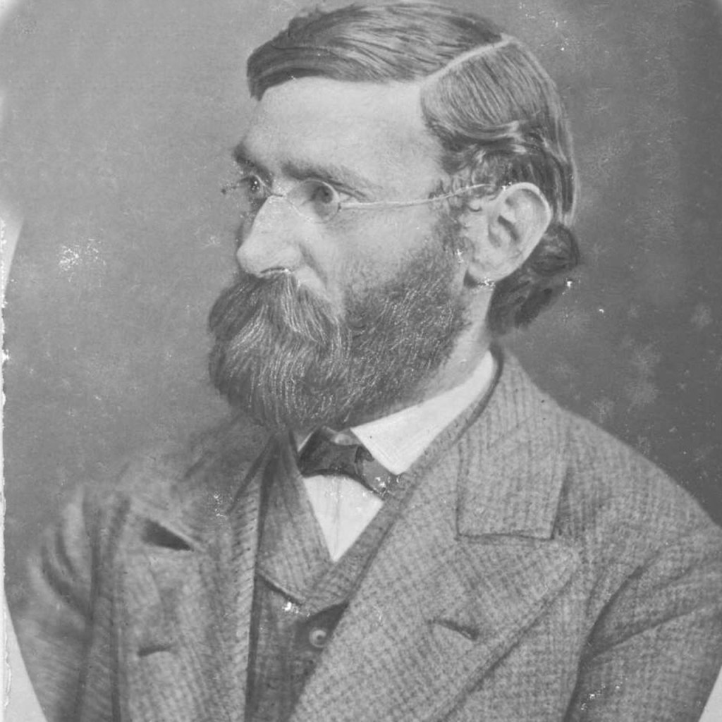
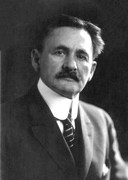
Michelson (1891): Astronomical Interferometry
Albert Michelson (1852 – 1931) was the first American to win the Nobel Prize in Physics. He received the award in 1907 for his work to replace the standard meter, based on a bar of metal housed in Paris, with the much more fundamental wavelength of red light emitted by Cadmium atoms. His work in Paris came on the heels of a new and surprising demonstration of the use of interferometry to measure the size of astronomical objects.
Albert Michelson
The wavelength of light (a millionth of a meter) seems ill-matched to measuring the size of astronomical objects (thousands of meters) that are so far from Earth (billions of meters). But this is where optical interferometry becomes so important. Michelson realized that light from a distant object, like a Galilean moon of Jupiter, would retain some partial coherence that could be measured using optical interferometry. Furthermore, by measuring how the interference depended on the separation of slits placed on the front of a telescope, it would be possible to determine the size of the astronomical object.
From left to right: Walter Adams, Albert Michelson, Walther Mayer, Albert Einstein, Max Ferrand, and Robert Milliken. Photo taken at Caltech.
In 1891, Michelson traveled to California where the Lick Observatory was poised high above the fog and dust of agricultural San Jose (a hundred years before San Jose became the capitol of high-tech Silicon Valley). Working with the observatory staff, he was able to make several key observations of the Galilean moons of Jupiter. These were just close enough that their sizes could be estimated (just barely) from conventional telescopes. Michelson found from his calculations of the interference effects that the sizes of the moons matched the conventional sizes to within reasonable error. This was the first demonstration of astronomical interferometry which has burgeoned into a huge sub-discipline of astronomy today—based originally on the Galilean moons [4].
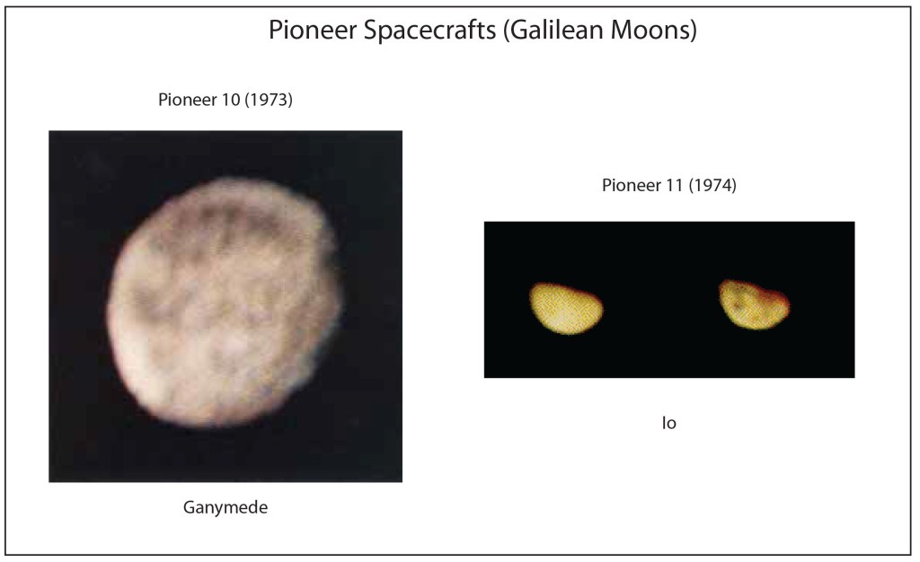
Pioneer (1973 – 1974): The First Tour
Pioneer 10 was launched on March 3, 1972 and made its closest approach to Jupiter on Dec. 3, 1973. Pioneer 11 was launched on April 5, 1973 and made its closest approach to Jupiter on Dec. 3, 1974 and later was the first spacecraft to fly by Saturn. The Pioneer spacecrafts were the first to leave the solar system (there have now been 5 that have left, or will leave, the solar system). The cameras on the Pioneers were single-pixel instruments that made line-scans as the spacecraft rotated. The point light detector was a Bendix Channeltron photomultiplier detector, which was a vacuum tube device (yes vacuum tube!) operating at a single-photon detection efficiency of around 10%. At the time of the system design, this was a state-of-the-art photon detector. The line scanning was sufficient to produce dramatic photographs (after extensive processing) of the giant planets. The much smaller moons were seen with low resolution, but were still the first close-ups ever to be made of Galileo’s moons.
Voyager (1979): The Grand Tour
Voyager 1 was launched on Sept. 5, 1977 and Voyager 2 was launched on August 20, 1977. Although Voyager 1 was launched second, it was the first to reach Jupiter with closest approach on March 5, 1979. Voyager 2 made its closest approach to Jupiter on July 9, 1979.
In the Fall of 1979, I had the good fortune to be an undergraduate at Cornell University when Carl Sagan gave an evening public lecture on the Voyager fly-bys, revealing for the first time the amazing photographs of not only Jupiter but of the Galilean Moons. Sitting in the audience listening to Sagan, a grand master of scientific story telling, made you feel like you were a part of history. I have never been so convinced of the beauty and power of science and technology as I was sitting in the audience that evening.
The camera technology on the Voyagers was a giant leap forward compared to the Pioneer spacecraft. The Voyagers used cathode ray vidicon cameras, like those used in television cameras of the day, with high-resolution imaging capabilities. The images were spectacular, displaying alien worlds in high-def for the first time in human history: volcanos and lava flows on the moon of Io; planet-long cracks in the ice-covered surface of Europa; Callisto’s pock-marked surface; Ganymede’s eerie colors.
The Voyager’s discoveries concerning the Galilean Moons were literally out of this world. Io was discovered to be a molten planet, its interior liquified by tidal-force heating from its nearness to Jupiter, spewing out sulfur lava onto a yellowed terrain pockmarked by hundreds of volcanoes, sporting mountains higher than Mt. Everest. Europa, by contrast, was discovered to have a vast flat surface of frozen ice, containing no craters nor mountains, yet fractured by planet-scale ruptures stained tan (for unknown reasons) against the white ice. Ganymede, the largest moon in the solar system, is a small planet, larger than Mercury. The Voyagers revealed that it had a blotchy surface with dark cratered patches interspersed with light smoother patches. Callisto, again by contrast, was found to be the most heavily cratered moon in the solar system, with its surface pocked by countless craters.
Galileo (1995): First in Orbit
The first mission to orbit Jupiter was the Galileo spacecraft that was launched, not from the Earth, but from Earth orbit after being delivered there by the Space Shuttle Atlantis on Oct. 18, 1989. Galileo arrived at Jupiter on Dec. 7, 1995 and was inserted into a highly elliptical orbit that became successively less eccentric on each pass. It orbited Jupiter for 8 years before it was purposely crashed into the planet (to prevent it from accidentally contaminating Europa that may support some form of life).
Galileo made many close passes to the Galilean Moons, providing exquisite images of the moon surfaces while its other instruments made scientific measurements of mass and composition. This was the first true extended study of Galileo’s Moons, establishing the likely internal structures, including the liquid water ocean lying below the frozen surface of Europa. As the largest body of liquid water outside the Earth, it has been suggested that some form of life could have evolved there (or possibly been seeded by meteor ejecta from Earth).
Juno (2016): Still Flying
The Juno spacecraft was launched from Cape Canaveral on Aug. 5, 2011 and entered a Jupiter polar orbit on July 5, 2016. The mission has been producing high-resolution studies of the planet. The mission was extended in 2021 to last to 2025 to include several close fly-bys of the Galilean Moons, especially Europa, which will be the object of several upcoming missions because of the possibility for the planet to support evolved life. These future missions include NASA’s Europa Clipper Mission, the ESA’s Jupiter Icy Moons Explorer, and the Io Volcano Observer.
Epilog (2060): Colonization of Callisto
In 2003, NASA identified the moon Callisto as the proposed site of a manned base for the exploration of the outer solar system. It would be the next most distant human base to be established after Mars, with a possible start date by the mid-point of this century. Callisto was chosen because it is has a low radiation level (being the farthest from Jupiter of the large moons) and is geologically stable. It also has a composition that could be mined to manufacture rocket fuel. The base would be a short-term way-station (crews would stay for no longer than a month) for refueling before launching and using a gravity assist from Jupiter to sling-shot spaceships to the outer planets.
By David D. Nolte, May 29, 2023
[1] See Chapter 2, A New Scientist: Introducing Galileo, in David D. Nolte, Galileo Unbound (Oxford University Press, 2018).
[2] Dava Sobel, Longitude: The True Story of a Lone Genius who Solved the Greatest Scientific Problem of his Time (Walker, 1995)
[3] See Chap. 1, Thomas Young Polymath: The Law of Interference, in David D. Nolte, Interference: The History of Optical Interferometry and the Scientists who Tamed Light (Oxford University Press, 2023)
[4] See Chapter 5, Stellar Interference: Measuring the Stars, in David D. Nolte, Interference: The History of Optical Interferometry and the Scientists who Tamed Light (Oxford University Press, 2023).
Read more in Books by David Nolte at Oxford University Press
An excerpt from the upcoming book “Interference: The History of Optical Interferometry and the Scientists who Tamed Light” describes how a handful of 19th-century scientists laid the groundwork for one of the key tools of modern optics. Published in Optics and Photonics News, March 2023.
François Arago rose to the highest levels of French science and politics. Along the way, he met Augustin Fresnel and, together, they changed the course of optical science.
Now is exactly the wrong moment to be reviewing the state of photonic quantum computing — the field is moving so rapidly, at just this moment, that everything I say here now will probably be out of date in just a few years. On the other hand, now is exactly the right time to be doing this review, because so much has happened in just the past few years, that it is important to take a moment and look at where this field is today and where it will be going.
At the 20-year anniversary of the publication of my book Mind at Light Speed (Free Press, 2001), this blog is the third in a series reviewing progress in three generations of Machines of Light over the past 20 years (see my previous blogs on the future of the photonic internet and on all-optical computers). This third and final update reviews progress on the third generation of the Machines of Light: the Quantum Optical Generation. Of the three generations, this is the one that is changing the fastest.
Quantum computing is almost here … and it will be at room temperature, using light, in photonic integrated circuits!
Quantum Computing with Linear Optics
Twenty years ago in 2001, Emanuel Knill and Raymond LaFlamme at Los Alamos National Lab, with Gerald Mulburn at the University of Queensland, Australia, published a revolutionary theoretical paper (known as KLM) in Nature on quantum computing with linear optics: “A scheme for efficient quantum computation with linear optics” [1]. Up until that time, it was believed that a quantum computer — if it was going to have the property of a universal Turing machine — needed to have at least some nonlinear interactions among qubits in a quantum gate. For instance, an example of a two-qubit gate is a controlled-NOT, or CNOT, gate shown in Fig. 1 with the Truth Table and the equivalent unitary matrix. It clear that one qubit is controlling the other, telling it what to do.
The quantum CNOT gate gets interesting when the control line has a quantum superposition, then the two outputs become entangled.
Entanglement is a strange process that is unique to quantum systems and has no classical analog. It also has no simple intuitive explanation. By any normal logic, if the control line passes through the gate unaltered, then absolutely nothing interesting should be happening on the Control-Out line. But that’s not the case. The control line going in was a separate state. If some measurement were made on it, either a 1 or 0 would be seen with equal probability. But coming out of the CNOT, the signal has somehow become perfectly correlated with whatever value is on the Signal-Out line. If the Signal-Out is measured, the measurement process collapses the state of the Control-Out to a value equal to the measured signal. The outcome of the control line becomes 100% certain even though nothing was ever done to it! This entanglement generation is one reason the CNOT is often the gate of choice when constructing quantum circuits to perform interesting quantum algorithms.
However, optical implementation of a CNOT is a problem, because light beams and photons really do not like to interact with each other. This is the problem with all-optical classical computers too (see my previous blog). There are ways of getting light to interact with light, for instance inside nonlinear optical materials. And in the case of quantum optics, a single atom in an optical cavity can interact with single photons in ways that can act like a CNOT or related gates. But the efficiencies are very low and the costs to implement it are very high, making it difficult or impossible to scale such systems up into whole networks needed to make a universal quantum computer.
Therefore, when KLM published their idea for quantum computing with linear optics, it caused a shift in the way people were thinking about optical quantum computing. A universal optical quantum computer could be built using just light sources, beam splitters and photon detectors.
The way that KLM gets around the need for a direct nonlinear interaction between two photons is to use postselection. They run a set of photons — signal photons and ancilla (test) photons — through their linear optical system and they detect (i.e., theoretically…the paper is purely a theoretical proposal) the ancilla photons. If these photons are not detected where they are wanted, then that iteration of the computation is thrown out, and it is tried again and again, until the photons end up where they need to be. When the ancilla outcomes are finally what they need to be, this run is selected because the signal state are known to have undergone a known transformation. The signal photons are still unmeasured at this point and are therefore in quantum superpositions that are useful for quantum computation. Postselection uses entanglement and measurement collapse to put the signal photons into desired quantum states. Postselection provides an effective nonlinearity that is induced by the wavefunction collapse of the entangled state. Of course, the down side of this approach is that many iterations are thrown out — the computation becomes non-deterministic.
KLM could get around most of the non-determinism by using more and more ancilla photons, but this has the cost of blowing up the size and cost of the implementation, so their scheme was not imminently practical. But the important point was that it introduced the idea of linear quantum computing. (For this, Milburn and his collaborators have my vote for a future Nobel Prize.) Once that idea was out, others refined it, and improved upon it, and found clever ways to make it more efficient and more scalable. Many of these ideas relied on a technology that was co-evolving with quantum computing — photonic integrated circuits (PICs).
Quantum Photonic Integrated Circuits (QPICs)
Never underestimate the power of silicon. The amount of time and energy and resources that have now been invested in silicon device fabrication is so astronomical that almost nothing in this world can displace it as the dominant technology of the present day and the future. Therefore, when a photon can do something better than an electron, you can guess that eventually that photon will be encased in a silicon chip–on a photonic integrated circuit (PIC).
The dream of integrated optics (the optical analog of integrated electronics) has been around for decades, where waveguides take the place of conducting wires, and interferometers take the place of transistors — all miniaturized and fabricated in the thousands on silicon wafers. The advantages of PICs are obvious, but it has taken a long time to develop. When I was a post-doc at Bell Labs in the late 1980’s, everyone was talking about PICs, but they had terrible fabrication challenges and terrible attenuation losses. Fortunately, these are just technical problems, not limited by any fundamental laws of physics, so time (and an army of researchers) has chipped away at them.
One of the driving forces behind the maturation of PIC technology is photonic fiber optic communications (as discussed in a previous blog). Photons are clear winners when it comes to long-distance communications. In that sense, photonic information technology is a close cousin to silicon — photons are no less likely to be replaced by a future technology than silicon is. Therefore, it made sense to bring the photons onto the silicon chips, tapping into the full array of silicon fab resources so that there could be seamless integration between fiber optics doing the communications and the photonic chips directing the information. Admittedly, photonic chips are not yet all-optical. They still use electronics to control the optical devices on the chip, but this niche for photonics has provided a driving force for advancements in PIC fabrication.
Fig. 2 Schematic of a silicon photonic integrated circuit (PIC). The waveguides can be silica or nitride deposited on the silicon chip. From the Comsol WebSite.
One side-effect of improved PIC fabrication is low light losses. In telecommunications, this loss is not so critical because the systems use OEO regeneration. But less loss is always good, and the PICs can now safeguard almost every photon that comes on chip — exactly what is needed for a quantum PIC. In a quantum photonic circuit, every photon is valuable and informative and needs to be protected. The new PIC fabrication can do this. In addition, light switches for telecom applications are built from integrated interferometers on the chip. It turns out that interferometers at the single-photon level are unitary quantum gates that can be used to build universal photonic quantum computers. So the same technology and control that was used for telecom is just what is needed for photonic quantum computers. In addition, integrated optical cavities on the PICs, which look just like wavelength filters when used for classical optics, are perfect for producing quantum states of light known as squeezed light that turn out to be valuable for certain specialty types of quantum computing.
Therefore, as the concepts of linear optical quantum computing advanced through that last 20 years, the hardware to implement those concepts also advanced, driven by a highly lucrative market segment that provided the resources to tap into the vast miniaturization capabilities of silicon chip fabrication. Very fortuitous!
Room-Temperature Quantum Computers
There are many radically different ways to make a quantum computer. Some are built of superconducting circuits, others are made from semiconductors, or arrays of trapped ions, or nuclear spins on nuclei on atoms in molecules, and of course with photons. Up until about 5 years ago, optical quantum computers seemed like long shots. Perhaps the most advanced technology was the superconducting approach. Superconducting quantum interference devices (SQUIDS) have exquisite sensitivity that makes them robust quantum information devices. But the drawback is the cold temperatures that are needed for them to work. Many of the other approaches likewise need cold temperature–sometimes astronomically cold temperatures that are only a few thousandths of a degree above absolute zero Kelvin.
Cold temperatures and quantum computing seemed a foregone conclusion — you weren’t ever going to separate them — and for good reason. The single greatest threat to quantum information is decoherence — the draining away of the kind of quantum coherence that allows interferences and quantum algorithms to work. In this way, entanglement is a two-edged sword. On the one hand, entanglement provides one of the essential resources for the exponential speed-up of quantum algorithms. But on the other hand, if a qubit “sees” any environmental disturbance, then it becomes entangled with that environment. The entangling of quantum information with the environment causes the coherence to drain away — hence decoherence. Hot environments disturb quantum systems much more than cold environments, so there is a premium for cooling the environment of quantum computers to as low a temperature as they can. Even so, decoherence times can be microseconds to milliseconds under even the best conditions — quantum information dissipates almost as fast as you can make it.
Enter the photon! The bottom line is that photons don’t interact. They are blind to their environment. This is what makes them perfect information carriers down fiber optics. It is also what makes them such good qubits for carrying quantum information. You can prepare a photon in a quantum superposition just by sending it through a lossless polarizing crystal, and then the superposition will last for as long as you can let the photon travel (at the speed of light). Sometimes this means putting the photon into a coil of fiber many kilometers long to store it, but that is OK — a kilometer of coiled fiber in the lab is no bigger than a few tens of centimeters. So the same properties that make photons excellent at carrying information also gives them very small decoherence. And after the KLM schemes began to be developed, the non-interacting properties of photons were no longer a handicap.
In the past 5 years there has been an explosion, as well as an implosion, of quantum photonic computing advances. The implosion is the level of integration which puts more and more optical elements into smaller and smaller footprints on silicon PICs. The explosion is the number of first-of-a-kind demonstrations: the first universal optical quantum computer [2], the first programmable photonic quantum computer [3], and the first (true) quantum computational advantage [4].
All of these “firsts” operate at room temperature. (There is a slight caveat: The photon-number detectors are actually superconducting wire detectors that do need to be cooled. But these can be housed off-chip and off-rack in a separate cooled system that is coupled to the quantum computer by — no surprise — fiber optics.) These are the advantages of photonic quantum computers: hundreds of qubits integrated onto chips, room-temperature operation, long decoherence times, compatibility with telecom light sources and PICs, compatibility with silicon chip fabrication, universal gates using postselection, and more. Despite the head start of some of the other quantum computing systems, photonics looks like it will be overtaking the others within only a few years to become the dominant technology for the future of quantum computing. And part of that future is being helped along by a new kind of quantum algorithm that is perfectly suited to optics.
Fig. 3 Superconducting photon counting detector. From WebSite
A New Kind of Quantum Algorithm: Boson Sampling
In 2011, Scott Aaronson (then at at MIT) published a landmark paper titled “The Computational Complexity of Linear Optics” with his post-doc, Anton Arkhipov [5]. The authors speculated on whether there could be an application of linear optics, not requiring the costly step of post-selection, that was still useful for applications, while simultaneously demonstrating quantum computational advantage. In other words, could one find a linear optical system working with photons that could solve problems intractable to a classical computer? To their own amazement, they did! The answer was something they called “boson sampling”.
To get an idea of what boson sampling is, and why it is very hard to do on a classical computer, think of the classic demonstration of the normal probability distribution found at almost every science museum you visit, illustrated in Fig. 2. A large number of ping-pong balls are dropped one at a time through a forest of regularly-spaced posts, bouncing randomly this way and that until they are collected into bins at the bottom. Bins near the center collect many balls, while bins farther to the side have fewer. If there are many balls, then the stacked heights of the balls in the bins map out a Gaussian probability distribution. The path of a single ping-pong ball represents a series of “decisions” as it hits each post and goes left or right, and the number of permutations of all the possible decisions among all the other ping-pong balls grows exponentially—a hard problem to tackle on a classical computer.
Fig. 4 Ping-pont ball normal distribution. Watch the YouTube video.
In the paper, Aaronson considered a quantum analog to the ping-pong problem in which the ping-pong balls are replaced by photons, and the posts are replaced by beam splitters. As its simplest possible implementation, it could have two photon channels incident on a single beam splitter. The well-known result in this case is the “HOM dip” [6] which is a consequence of the boson statistics of the photon. Now scale this system up to many channels and a cascade of beam splitters, and one has an N-channel multi-photon HOM cascade. The output of this photonic “circuit” is a sampling of the vast number of permutations allowed by bose statistics—boson sampling.
To make the problem more interesting, Aaronson allowed the photons to be launched from any channel at the top (as opposed to dropping all the ping-pong balls at the same spot), and they allowed each beam splitter to have adjustable phases (photons and phases are the key elements of an interferometer). By adjusting the locations of the photon channels and the phases of the beam splitters, it would be possible to “program” this boson cascade to mimic interesting quantum systems or even to solve specific problems, although they were not thinking that far ahead. The main point of the paper was the proposal that implementing boson sampling in a photonic circuit used resources that scaled linearly in the number of photon channels, while the problems that could be solved grew exponentially—a clear quantum computational advantage [4].
On the other hand, it turned out that boson sampling is not universal—one cannot construct a universal quantum computer out of boson sampling. The first proposal was a specialty algorithm whose main function was to demonstrate quantum computational advantage rather than do something specifically useful—just like Deutsch’s first algorithm. But just like Deutsch’s algorithm, which led ultimately to Shor’s very useful prime factoring algorithm, boson sampling turned out to be the start of a new wave of quantum applications.
Shortly after the publication of Aaronson’s and Arkhipov’s paper in 2011, there was a flurry of experimental papers demonstrating boson sampling in the laboratory [7, 8]. And it was discovered that boson sampling could solve important and useful problems, such as the energy levels of quantum systems, and network similarity, as well as quantum random-walk problems. Therefore, even though boson sampling is not strictly universal, it solves a broad class of problems. It can be viewed more like a specialty chip than a universal computer, like the now-ubiquitous GPU’s are specialty chips in virtually every desktop and laptop computer today. And the room-temperature operation significantly reduces cost, so you don’t need a whole government agency to afford one. Just like CPU costs followed Moore’s Law to the point where a Raspberry Pi computer costs $40 today, the photonic chips may get onto their own Moore’s Law that will reduce costs over the next several decades until they are common (but still specialty and probably not cheap) computers in academia and industry. A first step along that path was a recently-demonstrated general programmable room-temperature photonic quantum computer.
Fig. 5 A classical Galton board on the left, and a photon-based boson sampling on the right. From the Walmsley (Oxford) WebSite.
A Programmable Photonic Quantum Computer: Xanadu’s X8 Chip
I don’t usually talk about specific companies, but the new photonic quantum computer chip from Xanadu, based in Toronto, Canada, feels to me like the start of something big. In the March 4, 2021 issue of Nature magazine, researchers at the company published the experimental results of their X8 photonic chip [3]. The chip uses boson sampling of strongly non-classical light. This was the first generally programmable photonic quantum computing chip, programmed using a quantum programming language they developed called Strawberry Fields. By simply changing the quantum code (using a simple conventional computer interface), they switched the computer output among three different quantum applications: transitions among states (spectra of molecular states), quantum docking, and similarity between graphs that represent two different molecules. These are radically different physics and math problems, yet the single chip can be programmed on the fly to solve each one.
The chip is constructed of nitride waveguides on silicon, shown in Fig. 6. The input lasers drive ring oscillators that produce squeezed states through four-wave mixing. The key to the reprogrammability of the chip is the set of phase modulators that use simple thermal changes on the waveguides. These phase modulators are changed in response to commands from the software to reconfigure the application. Although they switch slowly, once they are set to their new configuration, the computations take place “at the speed of light”. The photonic chip is at room temperature, but the outputs of the four channels are sent by fiber optic to a cooled unit containing the superconductor nanowire photon counters.
Fig. 6 The Xanadu X8 photonic quantum computing chip. From Ref.Fig. 7 To see the chip in operation, see the YouTube video.
Admittedly, the four channels of the X8 chip are not large enough to solve the kinds of problems that would require a quantum computer, but the company has plans to scale the chip up to 100 channels. One of the challenges is to reduce the amount of photon loss in a multiplexed chip, but standard silicon fabrication approaches are expected to reduce loss in the next generation chips by an order of magnitude.
Additional companies are also in the process of entering the photonic quantum computing business, such as PsiQuantum, which recently closed a $450M funding round to produce photonic quantum chips with a million qubits. The company is led by Jeremy O’Brien from Bristol University who has been a leader in photonic quantum computing for over a decade.
[1] E. Knill, R. Laflamme, and G. J. Milburn, “A scheme for efficient quantum computation with linear optics,” Nature, vol. 409, no. 6816, pp. 46-52, Jan (2001)
[5] S. Aaronson and A. Arkhipov, “The Computational Complexity of Linear Optics,” in 43rd ACM Symposium on Theory of Computing, San Jose, CA, Jun 06-08 2011, NEW YORK: Assoc Computing Machinery, in Annual ACM Symposium on Theory of Computing, 2011, pp. 333-342
[8] M. A. Broome, A. Fedrizzi, S. Rahimi-Keshari, J. Dove, S. Aaronson, T. C. Ralph, and A. G. White, “Photonic Boson Sampling in a Tunable Circuit,” Science, vol. 339, no. 6121, pp. 794-798, Feb (2013)
Interference (New from Oxford University Press, 2023)
Read the stories of the scientists and engineers who tamed light and used it to probe the universe.
If you have ever seen euphemistically-named “snow”—the black and white dancing pixels on television screens in the old days of cathode-ray tubes—you may think it is nothing but noise. But the surprising thing about noise is that it is a good place to hide information.
Shine a laser pointer on any rough surface and look at the scattered light on a distant wall, then you will see the same patterns of light and dark known as laser speckle. If you move your head or move the pointer, then the speckle shimmers—just like the snow on the old TVs. This laser speckle—this snow—is providing fundamental new ways to extract information hidden inside three-dimensional translucent objects—objects like biological tissue or priceless paintings or silicon chips.
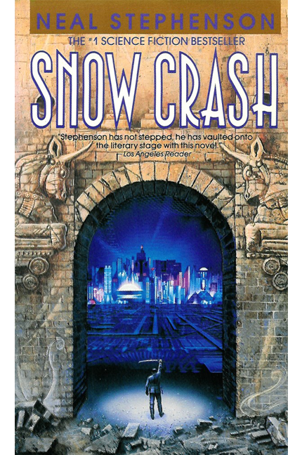
Snow Crash
The science fiction novel Snow Crash, published in 1992 by Neal Stephenson, is famous for popularizing virtual reality and the role of avatars. The central mystery of the novel is the mind-destroying mental crash that is induced by Snow—white noise in the metaverse. The protagonist hero of the story—a hacker with an avatar improbably named Hiro Protagonist—must find the source of snow and thwart the nefarious plot behind it.
Fig. 1 Book cover of Snow Crash
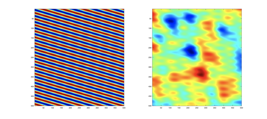
If Hiro’s snow in his VR headset is caused by laser speckle, then the seemingly random pattern is composed of amplitudes and phases that vary spatially and temporally. There are many ways to make computer-generated versions of speckle. One of the simplest is to just add together a lot of sinusoidal functions with varying orientations and periodicities. This is a “Fourier” approach to speckle which views it as a random superposition of two-dimensional spatial frequencies. An example is shown in Fig. 2 for one sinusoid which has been added to 20 others to generate the speckle pattern on the right. There is still residual periodicity in the speckle for N = 20, but as N increases, the speckle pattern becomes strictly random, like noise.
But if the sinusoids that are being added together link the periodicity with their amplitude through some functional relationship, then the final speckle can be analyze using a 2D Fourier transform to find its spatial frequency spectrum. The functional form of this spectrum can tell a lot about the underlying processes of the speckle formation. This is part of the information hidden inside snow.
Fig. 2 Sinusoidal addition to generate random speckle. a) One example of a spatial periodicity. b) The superposition of 20 random sinusoids.
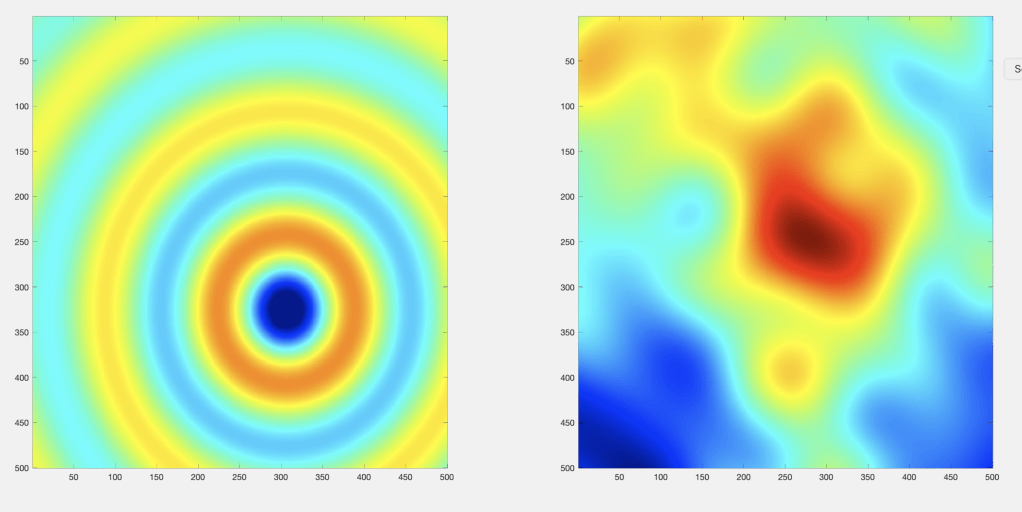
An alternative viewpoint to generating a laser speckle pattern thinks in terms of spatially-localized patches that add randomly together with random amplitudes and phases. This is a space-domain view of speckle formation in contrast to the Fourier-space view of the previous construction. Sinusoids are “global” extending spatially without bound. The underlying spatially localized functions can be almost any local function. Gaussians spring to mind, but so do Airy functions, because they are common point-spread functions that participate in the formation of images through lenses. The example in Fig 3a shows one such Airy function, and in 3b for speckle generated from N = 20 Airy functions of varying amplitudes and phases and locations.
Fig. 3 Generating speckle by random superposition of point spread functions (spatially-localized functions) of varying amplitude, phase, position and bandwidth.
These two examples are complementary ways of generating speckle, where the 2D Fourier-domain approach is conjugate to the 2D space-domain approach.
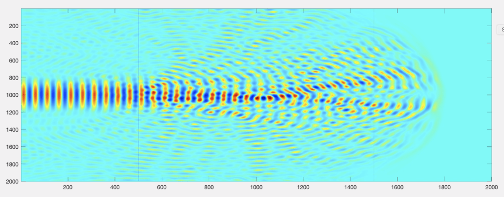
However, laser speckle is actually a 3D phenomenon, and the two-dimensional speckle patterns are just 2D cross sections intersecting a complex 3D pattern of light filaments. To get a sense of how laser speckle is formed in a physical system, one can solve the propagation of a laser beam through a random optical medium. In this way you can visualize the physical formation of the regions of brightness and darkness when the fragmented laser beam exits the random material.
Fig. 4 Propagation of a coherent beam into a random optical medium. Speckle is intrinsically three dimensional while 2D speckle is the cross section of the light filaments.
Coherent Patch
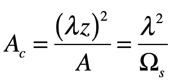
For a quantitative understanding of laser speckle, when 2D laser speckle is formed by an optical system, the central question is how big are the regions of brightness and darkness? This is a question of spatial coherence, and one way to define spatial coherence is through the coherence area at the observation plane
where A is the source emitting area, z is the distance to the observation plane, and Ωs is the solid angle subtended by the source emitting area as seen from the observation point. This expression assumes that the angular spread of the light scattered from the illumination area is very broad. Larger distances and smaller emitting areas (pinholes in an optical diffuser or focused laser spots on a rough surface) produce larger coherence areas in the speckle pattern. For a Gaussian intensity distribution at the emission plane, the coherence area is
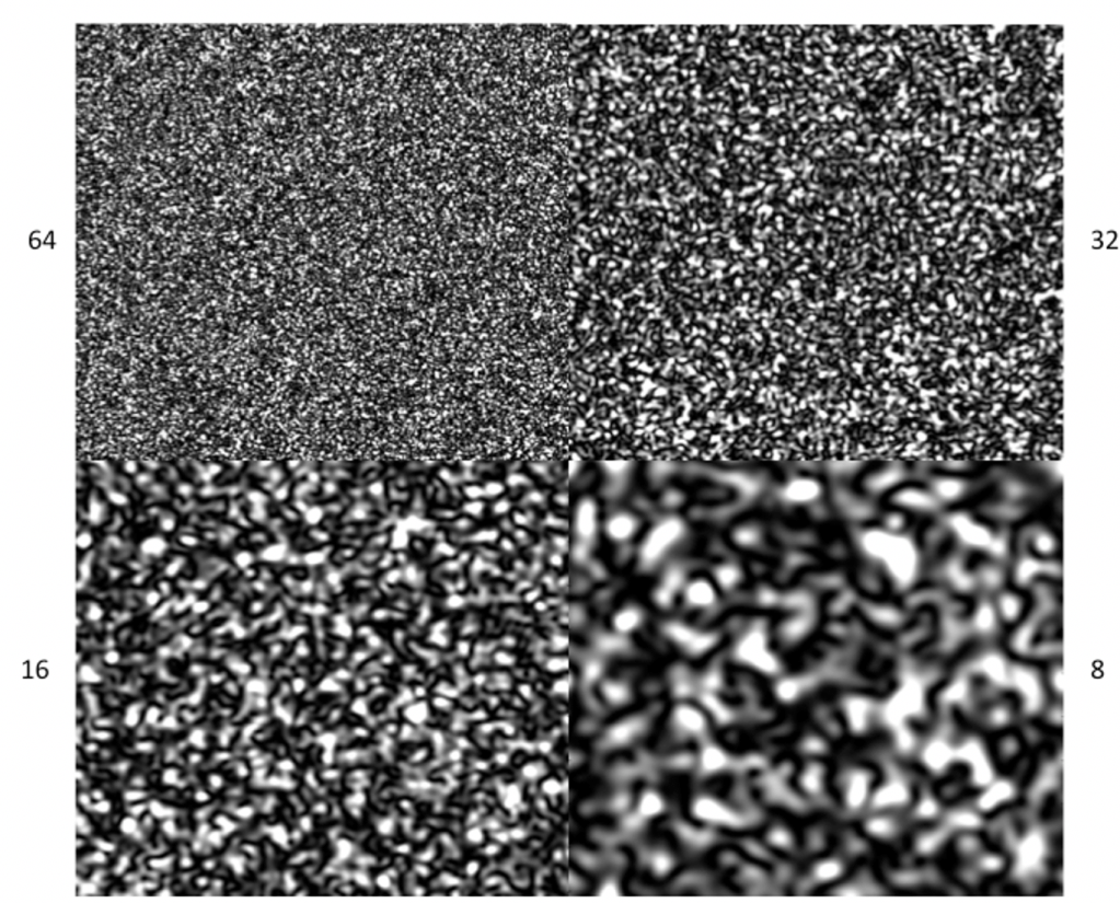
for beam waist w0 at the emission plane. To put some numbers to these parameters to give an intuitive sense of the size of speckle spots, assume a wavelength of 1 micron, a focused beam waist of 0.1 mm and a viewing distance of 1 meter. This gives patches with a radius of about 2 millimeters. Examples of laser speckle are shown in Fig. 5 for a variety of beam waist values w0.
Fig. 5 Speckle intensities for Gaussian illumination of a random phase screen for changing illumination radius w0 = 64, 32, 16 and 8 microns for f = 1 cm and W = 500 nm with a field-of-view of 5 mm. (Reproduced from Ref.[1])
Speckle Holograms
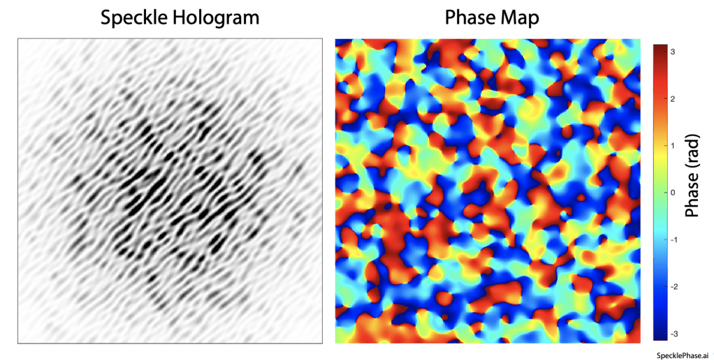
Associated with any intensity modulation must be a phase modulation through the Kramers-Kronig relations [2]. Phase cannot be detected directly in the speckle intensity pattern, but it can be measured by using interferometry. One of the easiest interferometric techniques is holography in which a coherent plane wave is caused to intersect, at a small angle, a speckle pattern generated from the same laser source. An example of a speckle hologram and its associated phase is shown in Fig. 6. The fringes of the hologram are formed when a plane reference wave interferes with the speckle field. The fringes are not parallel because of the varying phase of the speckle field, but the average spatial frequency is still recognizable in Fig. 5a. The associated phase map is shown in Fig. 5b.
Fig. 6 Speckle hologram and speckle phase. a) A coherent plane-wave reference added to fully-developed speckle (unity contrast) produces a speckle hologram. b) The phase of the speckle varies through 2π.
Optical Vortex Physics
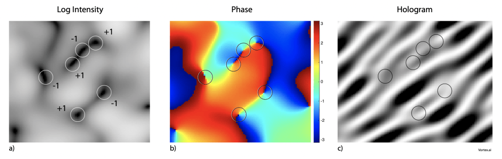
In the speckle intensity field, there are locations where the intensity vanishes, and the phase becomes undefined. In the neighborhood of a singular point the phase wraps around it with a 2pi phase range. Because of the wrapping phase such a singular point is called and optical vortex [3]. Vortices always come in pairs with opposite helicity (defined by the direction of the wrapping phase) with a line of neutral phase between them as shown in Fig. 7. The helicity defines the topological charge of the vortex, and they can have topological charges larger than ±1 if the phase wraps multiple times. In dynamic speckle these vortices are also dynamic and move with speeds related to the underlying dynamics of the scattering medium [4]. Vortices can annihilate if they have opposite helicity, and they can be created in pairs. Studies of singular optics have merged with structured illumination [5] to create an active field of topological optics with applications in biological microscopy as well as material science.
iFig. 7 Optical vortex patterns. a) Log intensity showing zeros in the intensity field. The circles identify the intensity nulls which are the optical vortices b) Associated phase with a 2pi phase wrapping around each singularity. c) Associated hologram showing dislocations in the fringes that occur at the vortices.
References
[1] D. D. Nolte, Optical Interferometry for Biology and Medicine. (Springer, 2012)
[2] A. Mecozzi, C. Antonelli, and M. Shtaif, “Kramers-Kronig coherent receiver,” Optica, vol. 3, no. 11, pp. 1220-1227, Nov (2016)
[3] M. R. Dennis, R. P. King, B. Jack, K. O’Holleran, and M. J. Padgett, “Isolated optical vortex knots,” Nature Physics, vol. 6, no. 2, pp. 118-121, Feb (2010)
[4] S. J. Kirkpatrick, K. Khaksari, D. Thomas, and D. D. Duncan, “Optical vortex behavior in dynamic speckle fields,” Journal of Biomedical Optics, vol. 17, no. 5, May (2012), Art no. 050504
[5] H. Rubinsztein-Dunlop, A. Forbes, M. V. Berry, M. R. Dennis, D. L. Andrews, M. Mansuripur, C. Denz, C. Alpmann, P. Banzer, T. Bauer, E. Karimi, L. Marrucci, M. Padgett, M. Ritsch-Marte, N. M. Litchinitser, N. P. Bigelow, C. Rosales-Guzman, A. Belmonte, J. P. Torres, T. W. Neely, M. Baker, R. Gordon, A. B. Stilgoe, J. Romero, A. G. White, R. Fickler, A. E. Willner, G. D. Xie, B. McMorran, and A. M. Weiner, “Roadmap on structured light,” Journal of Optics, vol. 19, no. 1, Jan (2017), Art no. 013001
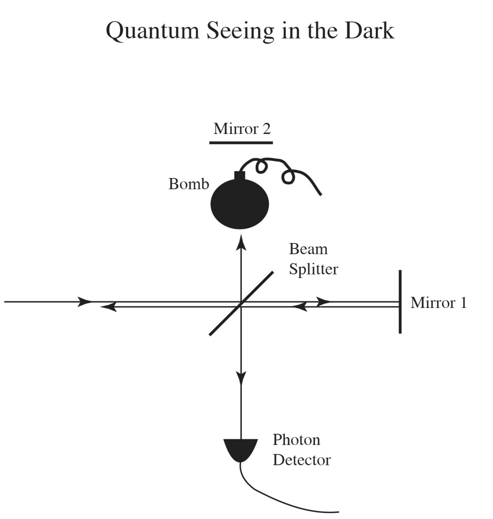
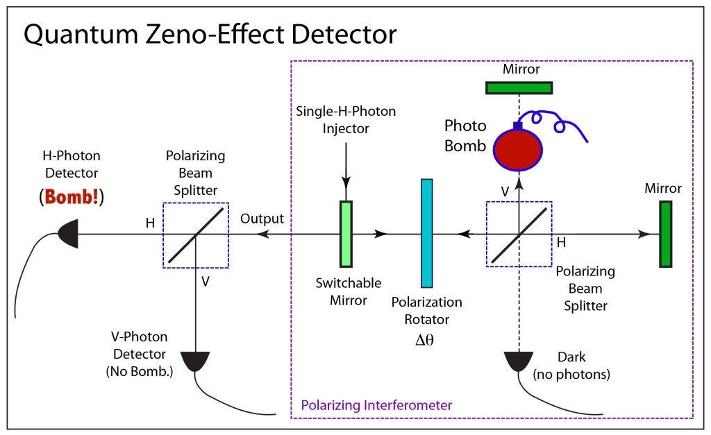
Quantum sensors have amazing powers. They can detect the presence of an obstacle without ever interacting with it. For instance, consider a bomb that is coated with a light sensitive layer that sets off the bomb if it absorbs just a single photon. Then put this bomb inside a quantum sensor system and shoot photons at it. Remarkably, using the weirdness of quantum mechanics, it is possible to design the system in such a way that you can detect the presence of the bomb using photons without ever setting it off. How can photons see the bomb without illuminating it? The answer is a bizarre side effect of quantum physics in which quantum wavefunctions are recognized as the root of reality as opposed to the pesky wavefunction collapse at the moment of measurement.
The ability for a quantum system to see an object with light, without exposing it, is uniquely a quantum phenomenon that has no classical analog.
All Paths Lead to Feynman
When Richard Feynman was working on his PhD under John Archibald Wheeler at Princeton in the early 1940’s he came across an obscure paper written by Paul Dirac in 1933 that connected quantum physics with classical Lagrangian physics. Dirac had recognized that the phase of a quantum wavefunction was analogous to the classical quantity called the “Action” that arises from Lagrangian physics. Building on this concept, Feynman constructed a new interpretation of quantum physics, known as the “many histories” interpretation, that occupies the middle ground between Schrödinger’s wave mechanics and Heisenberg’s matrix mechanics. One of the striking consequences of the many histories approach is the emergence of the principle of least action—a classical concept—into interpretations of quantum phenomena. In this approach, Feynman considered ALL possible histories for the propagation of a quantum particle from one point to another, he tabulated the quantum action in the phase factor, and he then summed all of these histories.
One of the simplest consequences of the sum over histories is a quantum interpretation of Snell’s law of refraction in optics. When summing over all possible trajectories of a photon from a point above to a point below an interface, there are a subset of paths for which the action integral varies very little from one path in the subset to another. The consequence of this is that the phases of all these paths add constructively, producing a large amplitude to the quantum wavefunction along the centroid of these trajectories. Conversely, for paths far away from this subset, the action integral takes on many values and the phases tend to interfere destructively, canceling the wavefunction along these other paths. Therefore, the most likely path of the photon between the two points is the path of maximum constructive interference and hence the path of stationary action. It is simple so show that this path is none other than the classical path determined by Snell’s Law and equivalently by Fermat’s principle of least time. With the many histories approach, we can add the principle of least (or stationary) action to the list of explanations of Snell’s Law. This argument holds as well for an electron (with mass and a de Broglie wavelength) as it does for a photon, so this not just a coincidence specific to optics but is a fundamental part of quantum physics.
A more subtle consequence of the sum over histories view of quantum phenomena is Young’s double slit experiment for electrons, shown at the top of Fig 1. The experiment consists of a source that emits only a single electron at a time that passes through a double-slit mask to impinge on an electron detection screen. The wavefunction for a single electron extends continuously throughout the full spatial extent of the apparatus, passing through both slits. When the two paths intersect at the screen, the difference in the quantum phases of the two paths causes the combined wavefunction to have regions of total constructive interference and other regions of total destructive interference. The probability of detecting an electron is proportional to the squared amplitude of the wavefunction, producing a pattern of bright stripes separated by darkness. At positions of destructive interference, no electrons are detected when both slits are open. However, if an opaque plate blocks the upper slit, then the interference pattern disappears, and electrons can be detected at those previously dark locations. Therefore, the presence of the object can be deduced by the detection of electrons at locations that should be dark.
Fig. 1 Demonstration of the sum over histories in a double-slit experiment for electrons. In the upper frame, the electron interference pattern on the phosphorescent screen produces bright and dark stripes. No electrons hit the screen in a dark stripe. When the upper slit is blocked (bottom frame), the interference pattern disappears, and an electron can arrive at the location that had previously been dark.
Consider now when the opaque plate is an electron-sensitive detector. In this case, a single electron emitted by the source can be detected at the screen or at the plate. If it is detected at the screen, it can appear at the location of a dark fringe, heralding the presence of the opaque plate. Yet the quantum conundrum is that when the electron arrives at a dark fringe, it must be detected there as a whole, it cannot be detected at the electron-sensitive plate too. So how does the electron sense the presence of the detector without exposing it, without setting it off?
In Feynman’s view, the electron does set off the detector as one possible history. And that history interferes with the other possible history when the electron arrives at the screen. While that interpretation may seem weird, mathematically it is a simple statement that the plate blocks the wavefunction from passing through the upper slit, so the wavefunction in front of the screen, resulting from all possible paths, has no interference fringes (other than possible diffraction from the lower slit). From this point of view, the wavefunction samples all of space, including the opaque plate, and the eventual absorption of a photon one place or another has no effect on the wavefunction. In this sense, it is the wavefunction, prior to any detection event, that samples reality. If the single electron happens to show up at a dark fringe at the screen, the plate, through its effects on the total wavefunction, has been detected without interacting with the photon.
This phenomenon is known as an interaction-free measurement, but there are definitely some semantics issues here. Just because the plate doesn’t absorb a photon, it doesn’t mean that the plate plays no role. The plate certainly blocks the wavefunction from passing through the upper slit. This might be called an “interaction”, but that phrase it better reserved for when the photon is actually absorbed, while the role of the plate in shaping the wavefunction is better described as one of the possible histories.
Quantum Seeing in the Dark
Although Feynman was thinking hard (and clearly) about these issues as he presented his famous lectures in physics at Cal Tech during 1961 to 1963, the specific possibility of interaction-free measurement dates more recently to 1993 when Avshalom C. Elitzur and Lev Vaidman at Tel Aviv University suggested a simple Michelson interferometer configuration that could detect an object half of the time without interacting with it [1]. They are the ones who first pressed this point home by thinking of a light-sensitive bomb. There is no mistaking when a bomb goes off, so it tends to give an exaggerated demonstration of the interaction-free measurement.
The Michelson interferometer for interaction-free measurement is shown in Fig. 2. This configuration uses a half-silvered beamsplitter to split the possible photon paths. When photons hit the beamsplitter, they either continue traveling to the right, or are deflected upwards. After reflecting off the mirrors, the photons again encounter the beamsplitter, where, in each case, they continue undeflected or are reflected. The result is that two paths combine at the beamsplitter to travel to the detector, while two other paths combine to travel back along the direction of the incident beam.
Fig. 2 A quantum-seeing in the dark (QSD) detector with a photo-sensitive bomb. A single photon is sent into the interferometer at a time. If the bomb is NOT present, destructive interference at the detector guarantees that the photon is not detected. However, if the bomb IS present, it destroys the destructive interference and the photon can arrive at the detector. That photon heralds the presence of the bomb without setting it off. (Reprinted from Mind @ Light Speed)
The paths of the light beams can be adjusted so that the beams that combine to travel to the detector experience perfect destructive interference. In this situation, the detector never detects light, and all the light returns back along the direction of the incident beam. Quantum mechanically, when only a single photon is present in the interferometer at a time, we would say that the quantum wavefunction of the photon interferes destructively along the path to the detector, and constructively along the path opposite to the incident beam, and the detector would detect no photons. It is clear that the unobstructed path of both beams results in the detector making no detections.
Now place the light sensitive bomb in the upper path. Because this path is no longer available to the photon wavefunction, the destructive interference of the wavefunction along the detector path is removed. Now when a single photon is sent into the interferometer, three possible things can happen. One, the photon is reflected by the beamsplitter and detonates the bomb. Two, the photon is transmitted by the beamsplitter, reflects off the right mirror, and is transmitted again by the beamsplitter to travel back down the incident path without being detected by the detector. Three, the photon is transmitted by the beamsplitter, reflects off the right mirror, and is reflected off the beamsplitter to be detected by the detector.
In this third case, the photon is detected AND the bomb does NOT go off, which succeeds at quantum seeing in the dark. The odds are much better than for Young’s experiment. If the bomb is present, it will detonate a maximum of 50% of the time. The other 50%, you will either detect a photon (signifying the presence of the bomb), or else you will not detect a photon (giving an ambiguous answer and requiring you to perform the experiment again). When you perform the experiment again, you again have a 50% chance of detonating the bomb, and a 25% chance of detecting it without it detonating, but again a 25% chance of not detecting it, and so forth. All in all, every time you send in a photon, you have one chance in four of seeing the bomb without detonating it. These are much better odds than for the Young’s apparatus where only exact detection of the photon at a forbidden location would signify the presence of the bomb.
It is possible to increase your odds above one chance in four by decreasing the reflectivity of the beamsplitter. In practice, this is easy to do simply by depositing less and less aluminum on the surface of the glass plate. When the reflectivity gets very low, let us say at the level of 1%, then most of the time the photon just travels back along the direction it came and you have an ambiguous result. On the other hand, when the photon does not return, there is an equal probability of detonation as detection. This means that, though you may send in many photons, your odds for eventually seeing the bomb without detonating it are nearly 50%, which is a factor of two better odds than for the half-silvered beamsplitter. A version of this experiment was performed by Paul Kwiat in 1995 as a postdoc at Innsbruck with Anton Zeilinger. It was Kwiat who coined the phrase “quantum seeing in the dark” as a catchier version of “interaction-free measurement” [2].
A 50% chance of detecting the bomb without setting it off sounds amazing, until you think that there is a 50% chance that it will go off and kill you. Then those odds don’t look so good. But optical phenomena never fail to surprise, and they never let you down. A crucial set of missing elements in the simple Michelson experiment was polarization-control using polarizing beamsplitters and polarization rotators. These are common elements in many optical systems, and when they are added to the Michelson quantum sensor, they can give almost a 100% chance of detecting the bomb without setting it off using the quantum Zeno effect.
The Quantum Zeno Effect
Photons carry polarization as their prime quantum number, with two possible orientations. These can be defined in different ways, but the two possible polarizations are orthogonal to each other. For instance, these polarization pairs can be vertical (V) and horizontal (H), or they can be right circular and left circular. One of the principles of quantum state evolution is that a quantum wavefunction can be maintained in a specific state, even if it has a tendency naturally to drift out of that state, by repeatedly making a quantum measurement that seeks to measure deviations from that state. In practice, the polarization of a photon can be maintained by repeatedly passing it through a polarizing beamsplitter with the polarization direction parallel to the original polarization of the photon. If there is a deviation in the photon polarization direction by a small angle, then a detector on the side port of the polarizing beamsplitter will fire with a probability equal to the square of the sine of the deviation. If the deviation angle is very small, say Δθ, then the probability of measuring the deviation is proportional to (Δθ)2, which is an even smaller number. Furthermore, the probability that the photon will transmit through the polarizing beamsplitter is equal to 1-(Δθ)2, which is nearly 100%.
This is what happens in Fig. 3 when the photo-sensitive bomb IS present. A single H-polarized photon is injected through a switchable mirror into the interferometer on the right. In the path of the photon is a polarization rotator that rotates the polarization by a small angle Δθ. There is nearly a 100% chance that the photon will transmit through the polarizing beamsplitter with perfect H-polarization reflect from the mirror and return through the polarizing beamsplitter, again with perfect H-polarization to pass through the polarization rotator to the switchable mirror where it reflects, gains another increment to its polarization angle, which is still small, and transmits through the beamsplitter, etc. At each pass, the photon polarization is repeatedly “measured” to be horizontal. After a number of passes N = π/Δθ/2, the photon is switched out of the interferometer and is transmitted through the external polarizing beamsplitter where it is detected at the H-photon detector.
Now consider what happens when the bomb IS NOT present. This time, even though there is a high amplitude for the transmitted photon, there is that Δθ amplitude for reflection out the V port. This small V-amplitude, when it reflects from the mirror, recombines with the H-amplitude at the polarizing beamsplitter to produce a polarization that has the same tilted polarizaton that it started with, sending it back in the direction from which it came. (In this situation, the detector on the “dark” port of the internal beamsplitter never sees the photon because of destructive interference along this path.) The photon is then rotated once more by the polarization rotator, and the photon polarization is rotated again, etc.. Now, after a number of passes N = π/Δθ/2, the photon has acquired a V polarization and is switched out of the interferometer. At the external polarizing beamsplitter it is reflected out of the V-port where it is detected at the V-photon detector.
Fig. 3 Quantum Zeno effect for interaction-free measurement. If the bomb is present, the H-photon detector detects the output photon without setting it off. The switchable mirror ejects the photon after it makes π/Δθ/2 round trips in the polarizing interferometer.
The two end results of this thought experiment are absolutely distinct, giving a clear answer to the question whether the bomb is present or not. If the bomb IS present, the H-detector fires. If the bomb IS NOT present, then the V-detector fires. Through all of this, the chance to set off the bomb is almost zero. Therefore, this quantum Zeno interaction-free measurement detects the bomb with nearly 100% efficiency with almost no chance of setting it off. This is the amazing consequence of quantum physics. The wavefunction is affected by the presence of the bomb, altering the interference effects that allow the polarization to rotate. But the likelihood of a photon being detected by the bomb is very low.
On a side note: Although ultrafast switchable mirrors do exist, the experiment was much easier to perform by creating a helix in the optical path through the system so that there is only a finite number of bounces of the photon inside the cavity. See Ref. [2] for details.
In conclusion, the ability for a quantum system to see an object with light, without exposing it, is uniquely a quantum phenomenon that has no classical analog. No E&M wave description can explain this effect.
Further Reading
I first wrote about quantum seeing the dark in my 2001 book on the future of optical physics and technology: Nolte, D. D. (2001). Mind at Light Speed : A new kind of intelligence. (New York, Free Press)
More on the story of Feynman and Wheeler and what they were trying to accomplish is told in Chapter 8 of Galileo Unbound on the physics and history of dynamics: Nolte, D. D. (2018). Galileo Unbound: A Path Across Life, the Universe and Everything (Oxford University Press).
Paul Kwiat introduced to the world to interaction-free measurements in 1995 in this illuminating Scientific American article: Kwiat, P., H. Weinfurter and A. Zeilinger (1996). “Quantum seeing in the dark – Quantum optics demonstrates the existence of interaction-free measurements: the detection of objects without light-or anything else-ever hitting them.” Scientific American 275(5): 72-78.
References
[1] Elitzur, A. C. and L. Vaidman (1993). “QUANTUM-MECHANICAL INTERACTION-FREE MEASUREMENTS.” Foundations of Physics 23(7): 987-997.
[2] Kwiat, P., H. Weinfurter, T. Herzog, A. Zeilinger and M. A. Kasevich (1995). “INTERACTION-FREE MEASUREMENT.” Physical Review Letters 74(24): 4763-4766.
In the midst of this COVID crisis (and the often botched governmental responses to it), there have been several success stories: Taiwan, South Korea, Australia and New Zealand stand out. What are the secrets to their success? First, is the willingness of the population to accept the seriousness of the pandemic and to act accordingly. Second, is a rapid and coherent (and competent) governmental response. Third, is biotechnology and the physics of ultra-sensitive biomolecule detection.
Antibody Testing
A virus consists a protein package called a capsid that surrounds polymers of coding RNA. Protein molecules on the capsid are specific to the virus and are the key to testing whether a person has been exposed to the virus. These specific molecules are called antigens, and the body produces antibodies — large biomolecules — that are rapidly evolved by the immune system and released into the blood system to recognize and bind to the antigen. The recognition and binding is highly specific (though not perfect) to the capsid proteins of the virus, so that other types of antibodies (produced to fend off other infections) tend not to bind to it. This specificity enables antibody testing.
In principle, all one needs to do is isolate the COVID-19 antigen, bind it to a surface, and run a sample of a patient’s serum (the part of the blood without the blood cells) over the same surface. If the patient has produced antibodies against the COVID-19, these antibodies will attach to the antigens stuck to the surface. After washing away the rest of the serum, what remains are anti-COVID antibodies attached to the antigens bound to the surface. The next step is to determine whether these antibodies have been bound to the surface or not.
Fig. 1 Schematic of an antibody macromolecule. The total height of the molecule is about 3 nanometers. The antigen binding sites are at the ends of the upper arms.
At this stage, there are many possible alternative technologies to detecting the bound antibodies (see section below on the physics of the BioCD for one approach). A conventional detection approach is known as ELISA (Enzyme-linked immunosorbant assay). To detect the bound antibody, a secondary antibody that binds to human antibodies is added to the test well. This secondary antibody contains either a fluorescent molecular tag or an enzyme that causes the color of the well to change (kind of like how a pregnancy test causes a piece of paper to change color). If the COVID antigen binds antibodies from the patient serum, then this second antibody will bind to the first and can be detected by fluorescence or by simple color change.
The technical challenges associated with antibody assays relate to false positives and false negatives. A false positive happens when the serum is too sticky and some antibodies NOT against COVID tend to stick to the surface of the test well. This is called non-specific binding. The secondary antibodies bind to these non-specifically-bound antibodies and a color change reports a detection, when in fact no COVID-specific antibodies were there. This is a false positive — the patient had not been exposed, but the test says they were.
On the other hand, a false negative occurs when the patient serum is possibly too dilute and even though anti-COVID antibodies are present, they don’t bind sufficiently to the test well to be detectable. This is a false negative — the patient had been exposed, but the test says they weren’t. Despite how mature antibody assay technology is, false positives and false negatives are very hard to eliminate. It is fairly common for false rates to be in the range of 5% to 10% even for high-quality immunoassays. The finite accuracy of the tests must be considered when doing community planning for testing and tracking. But the bottom line is that even 90% accuracy on the test can do a lot to stop the spread of the infection. This is because of the geometry of social networks and how important it is to find and isolate the super spreaders.
Social Networks
The web of any complex set of communities and their interconnections aren’t just random. Whether in interpersonal networks, or networks of cities and states and nations, it’s like the world-wide-web where the most popular webpages get the most links. This is the same phenomenon that makes the rich richer and the poor poorer. It produces a network with a few hubs that have a large fraction of the links. A network model that captures this network topology is known as the Barabasi-Albert model for scale-free networks [1]. A scale-free network tends to have one node that has the most links, then a couple of nodes that have a little fewer links, then several more with even fewer, and so on, until there are a vary large number of nodes with just a single link each.
When it comes to pandemics, this type of network topology is both a curse and a blessing. It is a curse, because if the popular node becomes infected it tends to infect a large fraction of the rest of the network because it is so linked in. But it is a blessing, because if that node can be identified and isolated from the rest of the network, then the chance of the pandemic sweeping across the whole network can be significantly reduced. This is where testing and contact tracing becomes so important. You have to know who is infected and who they are connected with. Only then can you isolate the central nodes of the network and make a dent in the pandemic spread.
An example of a Barabasi-Albert network is shown in Fig. 2 having 128 nodes. Some nodes have many links out (and in) the number of links connecting a node is called the node degree. There are several nodes of very high degree (a degree around 25 in this case) but also very many nodes that have only a single link. It’s the high-degree nodes that matter in a pandemic. If they get infected, then they infect almost the entire network. This scale-free network structure emphasizes the formation of central high-degree nodes. It tends to hold for many social networks, but also can stand for cities across a nation. A city like New York has links all over the country (by flights), while my little town of Lafayette IN might be modeled by a single link to Indianapolis. That same scaling structure is seen across many scales from interactions among nations to interactions among citizens in towns.
Fig. 2 A scale-free network with 128 nodes. A few nodes have high degree, but most nodes have a degree of one.
Isolating the Super Spreaders
In the network of nodes in Fig. 2, each node can be considered as a “compartment” in a multi-compartment SIR model (see my previous blog for the two-compartment SIR model of COVID-19). The infection of each node depends on the SIR dynamics of that node, plus the infections coming in from links other infected nodes. The equations of the dynamics for each node are
where Aab is the adjacency matrix where self-connection is allowed (infection dynamics within a node) and the sums go over all the nodes of the network. In this model, the population of each node is set equal to the degree ka of the node. The spread of the pandemic across the network depends on the links and where the infection begins, but the overall infection is similar to the simple SIR model for a given average network degree
However, if the pandemic starts, but then the highest-degree node (the super spreader) is isolated (by testing and contact tracing), then the saturation of the disease across the network can be decreased in a much greater proportion than simply given by the population of the isolated node. For instance, in the simulation in Fig. 3, a node of degree 20 is removed at 50 days. The fraction of the population that is isolated is only 10%, yet the saturation of the disease across the whole network is decreased by more than a factor of 2.
Fig. 3 Scale-free network of 128 nodes. Solid curve is infection dynamics of the full network. Dashed curve is the infection when the highest-degree node was isolated at 50 days.
In a more realistic model with many more nodes, and full testing to allow the infected nodes and their connections to be isolated, the disease can be virtually halted. This is what was achieved in Taiwan and South Korea. The question is why the United States, with its technologically powerful companies and all their capabilities, was so unprepared or unwilling to achieve the same thing.
Python Code: NetSIRSF.py
#!/usr/bin/env python3
# -*- coding: utf-8 -*-
"""
NetSIRSF.py
Created on Sat May 11 08:56:41 2019
@author: nolte
D. D. Nolte, Introduction to Modern Dynamics: Chaos, Networks, Space and Time, 2nd ed. (Oxford,2019)
"""

# https://www.python-course.eu/networkx.php
# https://networkx.github.io/documentation/stable/tutorial.html
# https://networkx.github.io/documentation/stable/reference/functions.html

import numpy as np
from scipy import integrate
from matplotlib import pyplot as plt
import networkx as nx
import time
from random import random

tstart = time.time()

plt.close('all')

betap = 0.014;
mu = 0.13;

print('beta = ',betap)
print('betap/mu = ',betap/mu)


N = 128      # 50


facoef = 2
k = 1
nodecouple = nx.barabasi_albert_graph(N, k, seed=None)

indhi = 0
deg = 0
for omloop in nodecouple.node:
    degtmp = nodecouple.degree(omloop)
    if degtmp > deg:
        deg = degtmp
        indhi = omloop
print('highest degree node = ',indhi)
print('highest degree = ',deg)

plt.figure(1)
colors = [(random(), random(), random()) for _i in range(10)]
nx.draw_circular(nodecouple,node_size=75, node_color=colors)
print(nx.info(nodecouple))

# function: omegout, yout = coupleN(G)
def coupleN(G,tlim):

    # function: yd = flow_deriv(x_y)
    def flow_deriv(x_y,t0):

        N = np.int(x_y.size/2)
        yd = np.zeros(shape=(2*N,))
        ind = -1
        for omloop in G.node:
            ind = ind + 1
            temp1 = -mu*x_y[ind] + betap*x_y[ind]*x_y[N+ind]
            temp2 =  -betap*x_y[ind]*x_y[N+ind]
            linksz = G.node[omloop]['numlink']
            for cloop in range(linksz):
                cindex = G.node[omloop]['link'][cloop]
                indx = G.node[cindex]['index']
                g = G.node[omloop]['coupling'][cloop]

                temp1 = temp1 + g*betap*x_y[indx]*x_y[N+ind]
                temp2 = temp2 - g*betap*x_y[indx]*x_y[N+ind]

            yd[ind] = temp1
            yd[N+ind] = temp2

        return yd
    # end of function flow_deriv(x_y)
    x0 = x_y
    t = np.linspace(0,tlim,tlim)      # 600  300
    y = integrate.odeint(flow_deriv, x0, t)

    return t,y
    # end of function: omegout, yout = coupleN(G)

lnk = np.zeros(shape = (N,), dtype=int)
ind = -1
for loop in nodecouple.node:
    ind = ind + 1
    nodecouple.node[loop]['index'] = ind
    nodecouple.node[loop]['link'] = list(nx.neighbors(nodecouple,loop))
    nodecouple.node[loop]['numlink'] = len(list(nx.neighbors(nodecouple,loop)))
    lnk[ind] = len(list(nx.neighbors(nodecouple,loop)))

gfac = 0.1

ind = -1
for nodeloop in nodecouple.node:
    ind = ind + 1
    nodecouple.node[nodeloop]['coupling'] = np.zeros(shape=(lnk[ind],))
    for linkloop in range (lnk[ind]):
        nodecouple.node[nodeloop]['coupling'][linkloop] = gfac*facoef

x_y = np.zeros(shape=(2*N,))
for loop in nodecouple.node:
    x_y[loop]=0
    x_y[N+loop]=nodecouple.degree(loop)
    #x_y[N+loop]=1
x_y[N-1 ]= 0.01
x_y[2*N-1] = x_y[2*N-1] - 0.01
N0 = np.sum(x_y[N:2*N]) - x_y[indhi] - x_y[N+indhi]
print('N0 = ',N0)

tlim0 = 600
t0,yout0 = coupleN(nodecouple,tlim0)                           # Here is the subfunction call for the flow


plt.figure(2)
plt.yscale('log')
plt.gca().set_ylim(1e-3, 1)
for loop in range(N):
    lines1 = plt.plot(t0,yout0[:,loop])
    lines2 = plt.plot(t0,yout0[:,N+loop])
    lines3 = plt.plot(t0,N0-yout0[:,loop]-yout0[:,N+loop])

    plt.setp(lines1, linewidth=0.5)
    plt.setp(lines2, linewidth=0.5)
    plt.setp(lines3, linewidth=0.5)


Itot = np.sum(yout0[:,0:127],axis = 1) - yout0[:,indhi]
Stot = np.sum(yout0[:,128:255],axis = 1) - yout0[:,N+indhi]
Rtot = N0 - Itot - Stot
plt.figure(3)
#plt.plot(t0,Itot,'r',t0,Stot,'g',t0,Rtot,'b')
plt.plot(t0,Itot/N0,'r',t0,Rtot/N0,'b')
#plt.legend(('Infected','Susceptible','Removed'))
plt.legend(('Infected','Removed'))
plt.hold

# Repeat but innoculate highest-degree node
x_y = np.zeros(shape=(2*N,))
for loop in nodecouple.node:
    x_y[loop]=0
    x_y[N+loop]=nodecouple.degree(loop)
    #x_y[N+loop]=1
x_y[N-1] = 0.01
x_y[2*N-1] = x_y[2*N-1] - 0.01
N0 = np.sum(x_y[N:2*N]) - x_y[indhi] - x_y[N+indhi]

tlim0 = 50
t0,yout0 = coupleN(nodecouple,tlim0)


# remove all edges from highest-degree node
ee = list(nodecouple.edges(indhi))
nodecouple.remove_edges_from(ee)
print(nx.info(nodecouple))

#nodecouple.remove_node(indhi)
lnk = np.zeros(shape = (N,), dtype=int)
ind = -1
for loop in nodecouple.node:
    ind = ind + 1
    nodecouple.node[loop]['index'] = ind
    nodecouple.node[loop]['link'] = list(nx.neighbors(nodecouple,loop))
    nodecouple.node[loop]['numlink'] = len(list(nx.neighbors(nodecouple,loop)))
    lnk[ind] = len(list(nx.neighbors(nodecouple,loop)))

ind = -1
x_y = np.zeros(shape=(2*N,))
for nodeloop in nodecouple.node:
    ind = ind + 1
    nodecouple.node[nodeloop]['coupling'] = np.zeros(shape=(lnk[ind],))
    x_y[ind] = yout0[tlim0-1,nodeloop]
    x_y[N+ind] = yout0[tlim0-1,N+nodeloop]
    for linkloop in range (lnk[ind]):
        nodecouple.node[nodeloop]['coupling'][linkloop] = gfac*facoef


tlim1 = 500
t1,yout1 = coupleN(nodecouple,tlim1)

t = np.zeros(shape=(tlim0+tlim1,))
yout = np.zeros(shape=(tlim0+tlim1,2*N))
t[0:tlim0] = t0
t[tlim0:tlim1+tlim0] = tlim0+t1
yout[0:tlim0,:] = yout0
yout[tlim0:tlim1+tlim0,:] = yout1


plt.figure(4)
plt.yscale('log')
plt.gca().set_ylim(1e-3, 1)
for loop in range(N):
    lines1 = plt.plot(t,yout[:,loop])
    lines2 = plt.plot(t,yout[:,N+loop])
    lines3 = plt.plot(t,N0-yout[:,loop]-yout[:,N+loop])

    plt.setp(lines1, linewidth=0.5)
    plt.setp(lines2, linewidth=0.5)
    plt.setp(lines3, linewidth=0.5)


Itot = np.sum(yout[:,0:127],axis = 1) - yout[:,indhi]
Stot = np.sum(yout[:,128:255],axis = 1) - yout[:,N+indhi]
Rtot = N0 - Itot - Stot
plt.figure(3)
#plt.plot(t,Itot,'r',t,Stot,'g',t,Rtot,'b',linestyle='dashed')
plt.plot(t,Itot/N0,'r',t,Rtot/N0,'b',linestyle='dashed')
#plt.legend(('Infected','Susceptible','Removed'))
plt.legend(('Infected','Removed'))
plt.xlabel('Days')
plt.ylabel('Fraction of Sub-Population')
plt.title('Network Dynamics for COVID-19')
plt.show()
plt.hold()

elapsed_time = time.time() - tstart
print('elapsed time = ',format(elapsed_time,'.2f'),'secs')
Caveats and Disclaimers
No effort in the network model was made to fit actual disease statistics. In addition, the network in Figs. 2 and 3 only has 128 nodes, and each node was a “compartment” that had its own SIR dynamics. This is a coarse-graining approach that would need to be significantly improved to try to model an actual network of connections across communities and states. In addition, isolating the super spreader in this model would be like isolating a city rather than an individual, which is not realistic. The value of a heuristic model is to gain a physical intuition about scales and behaviors without being distracted by details of the model.
Postscript: Physics of the BioCD
Because antibody testing has become such a point of public discussion, it brings to mind a chapter of my own life that was closely related to this topic. About 20 years ago my research group invented and developed an antibody assay called the BioCD [2]. The “CD” stood for “compact disc”, and it was a spinning-disk format that used laser interferometry to perform fast and sensitive measurements of antibodies in blood. We launched a start-up company called QuadraSpec in 2004 to commercialize the technology for large-scale human disease screening.
A conventional compact disc consists of about a billion individual nulling interferometers impressed as pits into plastic. When the read-out laser beam straddles one of the billion pits, it experiences a condition of perfect destructive interferences — a zero. But when it was not shining on a pit it experiences high reflection — a one. So as the laser scans across the surface of the disc as it spins, a series of high and low reflections read off bits of information. Because the disc spins very fast, the data rate is very high, and a billion bits can be read in a matter of minutes.
The idea struck me in late 1999 just before getting on a plane to spend a weekend in New York City: What if each pit were like a test tube, so that instead of reading bits of ones and zeros it could read tiny amounts of protein? Then instead of a billion ones and zeros the disc could read a billion protein concentrations. But nulling interferometers are the least sensitive way to measure something sensitively because it operates at a local minimum in the response curve. The most sensitive way to do interferometry is in the condition of phase quadrature when the signal and reference waves are ninety-degrees out of phase and where the response curve is steepest, as in Fig. 4 . Therefore, the only thing you need to turn a compact disc from reading ones and zeros to proteins is to reduce the height of the pit by half. In practice we used raised ridges of gold instead of pits, but it worked in the same way and was extremely sensitive to the attachment of small amounts of protein.
Fig. 4 Principle of the BioCD antibody assay. Reprinted from Ref. [3]
This first generation BioCD was literally a work of art. It was composed of a radial array of gold strips deposited on a silicon wafer. We were approached in 2004 by an art installation called “Massive Change” that was curated by the Vancouver Art Museum. The art installation travelled to Toronto and then to the Museum of Contemporary Art in Chicago, where we went to see it. Our gold-and-silicon BioCD was on display in a section on art in technology.
The next-gen BioCDs were much simpler, consisting simply of oxide layers on silicon wafers, but they were much more versatile and more sensitive. An optical scan of a printed antibody spot on a BioCD is shown in Fig. 5 The protein height is only about 1 nanometer (the diameter of the spot is 100 microns). Interferometry can measure a change in the height of the spot (caused by binding antibodies from patient serum) by only about 10 picometers averaged over the size of the spot. This exquisite sensitivity enabled us to detect tiny fractions of blood-born antigens and antibodies at the level of only a nanogram per milliliter.
Fig. 5 Interferometric measurement of a printed antibody spot on a BioCD. The spot height is about 1 nanomater and the diameter is about 100 microns. Interferometry can measure a change of height by about 10 picometers averaged over the spot.
The real estate on a 100 mm diameter disc was sufficient to do 100,000 antibody assays, which would be 256 protein targets across 512 patients on a single BioCD that would take only a few hours to finish reading!
Fig. 6 A single BioCD has the potential to measure hundreds of proteins or antibodies per patient with hundreds of patients per disc.
The potential of the BioCD for massively multiplexed protein measurements made it possible to imagine testing a single patient for hundreds of diseases in a matter of hours using only a few drops of blood. Furthermore, by being simple and cheap, the test would allow people to track their health over time to look for emerging health trends.
If this sounds familiar to you, you’re right. That’s exactly what the notorious company Theranos was promising investors 10 years after we first proposed this idea. But here’s the difference: We learned that the tech did not scale. It cost us $10M to develop a BioCD that could test for just 4 diseases. And it would cost more than an additional $10M to get it to 8 diseases, because the antibody chemistry is not linear. Each new disease that you try to test creates a combinatorics problem of non-specific binding with all the other antibodies and antigens. To scale the test up to 100 diseases on the single platform using only a few drops of blood would have cost us more than $1B of R&D expenses — if it was possible at all. So we stopped development at our 4-plex product and sold the technology to a veterinary testing company that uses it today to test for diseases like heart worm and Lymes disease in blood samples from pet animals.
Five years after we walked away from massively multiplexed antibody tests, Theranos proposed the same thing and took in more than $700M in US investment, but ultimately produced nothing that worked. The saga of Theranos and its charismatic CEO Elizabeth Holmes has been the topic of books and documentaries and movies like “The Inventor: Out for Blood in Silicon Valley” and a rumored big screen movie starring Jennifer Lawrence as Holmes.
The bottom line is that antibody testing is a difficult business, and ramping up rapidly to meet the demands of testing and tracing COVID-19 is going to be challenging. The key is not to demand too much accuracy per test. False positives are bad for the individual, because it lets them go about without immunity and they might get sick, and false negatives are bad, because it locks them in when they could be going about. But if an inexpensive test of only 90% accuracy (a level of accuracy that has already been called “unreliable” in some news reports) can be brought out in massive scale so that virtually everyone can be tested, and tested repeatedly, then the benefit to society would be great. In the scaling networks that tend to characterize human interactions, all it takes is a few high-degree nodes to be isolated to make infection rates plummet.
References
[1] A. L. Barabasi and R. Albert, “Emergence of scaling in random networks,” Science, vol. 286, no. 5439, pp. 509-512, Oct 15 (1999)
[2] D. D. Nolte, “Review of centrifugal microfluidic and bio-optical disks,” Review Of Scientific Instruments, vol. 80, no. 10, p. 101101, Oct (2009)
[3] D. D. Nolte and F. E. Regnier, “Spinning-Disk Interferometry: The BioCD,” Optics and Photonics News, no. October 2004, pp. 48-53, (2004)