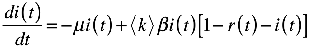
These days, the physics breakthroughs in the news that really catch the eye tend to be Astro-centric. Partly, this is due to the new data coming from the James Webb Space Telescope, which is the flashiest and newest toy of the year in physics. But also, this is part of a broader trend in physics that we see in the interest statements of physics students applying to graduate school. With the Higgs business winding down for high energy physics, and solid state physics becoming more engineering, the frontiers of physics have pushed to the skies, where there seem to be endless surprises.
To be sure, quantum information physics (a hot topic) and AMO (atomic and molecular optics) are performing herculean feats in the laboratories. But even there, Bose-Einstein condensates are simulating the early universe, and quantum computers are simulating worm holes—tipping their hat to astrophysics!
So here are my picks for the top physics breakthroughs of 2023.
The Early Universe
The James Webb Space Telescope (JWST) has come through big on all of its promises! They said it would revolutionize the astrophysics of the early universe, and they were right. As of 2023, all astrophysics textbooks describing the early universe and the formation of galaxies are now obsolete, thanks to JWST.
Foremost among the discoveries is how fast the universe took up its current form. Galaxies condensed much earlier than expected, as did supermassive black holes. Everything that we thought took billions of years seem to have happened in only about one-tenth of that time (incredibly fast on cosmic time scales). The new JWST observations blow away the status quo on the early universe, and now the astrophysicists have to go back to the chalk board.
If LIGO and the first detection of gravitational waves was the huge breakthrough of 2015, detecting something so faint that it took a century to build an apparatus sensitive enough to detect them, then the newest observations of gravitational waves using galactic ripples presents a whole new level of gravitational wave physics.
By using the exquisitely precise timing of distant pulsars, astrophysicists have been able to detect a din of gravitational waves washing back and forth across the universe. These waves came from supermassive black hole mergers in the early universe. As the waves stretch and compress the space between us and distant pulsars, the arrival times of pulsar pulses detected at the Earth vary a tiny but measurable amount, haralding the passing of a gravitational wave.
This approach is a form of statistical optics in contrast to the original direct detection that was a form of interferometry. These are complimentary techniques in optics research, just as they will be complimentary forms of gravitational wave astronomy. Statistical optics (and fluctuation analysis) provides spectral density functions which can yield ensemble averages in the large N limit. This can answer questions about large ensembles that single interferometric detection cannot contribute to. Conversely, interferometric detection provides the details of individual events in ways that statistical optics cannot do. The two complimentary techniques, moving forward, will provide a much clearer picture of gravitational wave physics and the conditions in the universe that generate them.
Phosphorous on Enceladus
Planetary science is the close cousin to the more distant field of cosmology, but being close to home also makes it more immediate. The search for life outside the Earth stands as one of the greatest scientific quests of our day. We are almost certainly not alone in the universe, and life may be as close as Enceladus, the icy moon of Saturn.
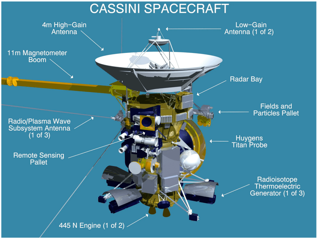
Scientists have been studying data from the Cassini spacecraft that observed Saturn close-up for over a decade from 2004 to 2017. Enceladus has a subsurface liquid ocean that generates plumes of tiny ice crystals that erupt like geysers from fissures in the solid surface. The ocean remains liquid because of internal tidal heating caused by the large gravitational forces of Saturn.
The Cassini spacecraft flew through the plumes and analyzed their content using its Cosmic Dust Analyzer. While the ice crystals from Enceladus were already known to contain organic compounds, the science team discovered that they also contain phosphorous. This is the least abundant element within the molecules of life, but it is absolutely essential, providing the backbone chemistry of DNA as well as being a constituent of amino acids.
With this discovery, all the essential building blocks of life are known to exist on Enceladus, along with a liquid ocean that is likely to be in chemical contact with rocky minerals on the ocean floor, possibly providing the kind of environment that could promote the emergence of life on a planet other than Earth.
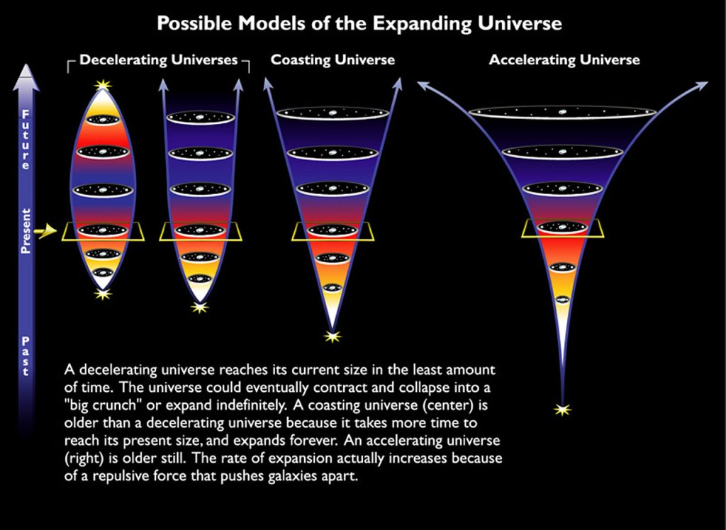
Simulating the Expanding Universe in a Bose-Einstein Condensate
Putting the universe under a microscope in a laboratory may have seemed a foolish dream, until a group at the University of Heidelberg did just that. It isn’t possible to make a real universe in the laboratory, but by adjusting the properties of an ultra-cold collection of atoms known as a Bose-Einstein condensate, the research group was able to create a type of local space whose internal metric has a curvature, like curved space-time. Furthermore, by controlling the inter-atomic interactions of the condensate with a magnetic field, they could cause the condensate to expand or contract, mimicking different scenarios for the evolution of our own universe. By adjusting the type of expansion that occurs, the scientists could create hypotheses about the geometry of the universe and test them experimentally, something that could never be done in our own universe. This could lead to new insights into the behavior of the early universe and the formation of its large-scale structure.
This is the only breakthrough I picked that is not related to astrophysics (although even this effect may have played a role in the very early universe).
Entanglement is one of the hottest topics in physics today (although the idea is 89 years old) because of the crucial role it plays in quantum information physics. The topic was awarded the 2022 Nobel Prize in Physics which went to John Clauser, Alain Aspect and Anton Zeilinger.
Direct observations of entanglement have been mostly restricted to optics (where entangled photons are easily created and detected) or molecular and atomic physics as well as in the solid state.
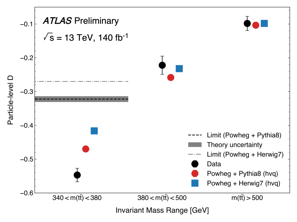
But entanglement eluded high-energy physics (which is quantum matter personified) until 2023 when the Atlas Collaboration at the LHC (Large Hadron Collider) in Geneva posted a manuscript on Arxiv that reported the first observation of entanglement in the decay products of a quark.
Fig. Thresholds for entanglement detection in decays from top quarks. Imagecredit.
Quarks interact so strongly (literally through the strong force), that entangled quarks experience very rapid decoherence, and entanglement effects virtually disappear in their decay products. However, top quarks decay so rapidly, that their entanglement properties can be transferred to their decay products, producing measurable effects in the downstream detection. This is what the Atlas team detected.
While this discovery won’t make quantum computers any better, it does open up a new perspective on high-energy particle interactions, and may even have contributed to the properties of the primordial soup during the Big Bang.
Something strange almost happened in 1840’s England just a few years into Queen Victoria’s long reign—a giant machine the size of a large shed, built of thousands of interlocking steel gears, driven by steam power, almost came to life—a thinking, mechanical automaton, the very image of Cyber Steampunk.
Cyber Steampunk is a genre of media that imagines an alternate history of a Victorian Age with advanced technology—airships and rockets and robots and especially computers—driven by steam power. Some of the classics that helped launch the genre are the animé movies Castle in the Sky (1986) by Hayao Miyazaki and Steam Boy (2004) by Katsuhiro Otomo and the novel The Difference Engine (1990) by William Gibson and Bruce Sterling. The novel pursues Ada Byron, Lady Lovelace, through the shadows of London by those who suspect she has devised a programmable machine that can win at gambling using steam and punched cards. This is not too far off from what might have happened in real life if Ada Lovelace had a bit more sway over one of her unsuitable suitors—Charles Babbage.
But Babbage, part genius, part fool, could not understand what Lovelace understood—for if he had, a Victorian computer built of oiled gears and leaky steam pipes, instead of tiny transistors and metallic leads, might have come a hundred years early as another marvel of the already marvelous Industrial Revolution. How might our world today be different if Babbage had seen what Lovelace saw?
There is no question of Babbage’s genius. He was so far ahead of his time that he appeared to most people in his day to be a crackpot, and he was often treated as one. His father thought he was useless, and he told him so, because to be a scientist in the early 1800’s was to be unemployable, and Babbage was unemployed for years after college. Science was, literally, natural philosophy, and no one hired a philosopher unless they were faculty at some college. But Babbage’s friends from Trinity College, Cambridge, like William Whewell (future dean of Trinity) and John Herschel (son of the famous astronomer), new his worth and were loyal throughout their lives and throughout his trials.
Fig. 2 Charles Babbage
Charles Babbage was a favorite at Georgian dinner parties because he was so entertaining to watch and to listen to. From personal letters of his friends (and enemies) of the time one gets a picture of a character not too different from Sheldon Cooper on the TV series The Big Bang Theory—convinced of his own genius and equally convinced of the lack of genius of everyone else and ready to tell them so. His mind was so analytic, that he talked like a walking computer—although nothing like a computer existed in those days—everything was logic and functions and propositions—hence his entertainment value. No one understood him, and no one cared—until he ran into a young woman who actually did, but more of that later.
One summer day in 1821, Babbage and Herschel were working on mathematical tables for the Astrophysical Society, a dull but important job to ensure that star charts and moon positions could be used accurately for astronomical calculations and navigation. The numbers filled column after column, page after page. But as they checked the values, the two were shocked by how many entries in the tables were wrong. In that day, every numerical value of every table or chart was calculated by a person (literally called a computer), and people make mistakes. Even as they went to correct the numbers, new mistakes would crop in. In frustration, Babbage exclaimed to Herschel that what they needed was a steam-powered machine that would calculate the numbers automatically. No sooner had he said it, than Babbage had a vision of a mechanical machine, driven by a small steam engine, full of gears and rods, that would print out the tables automatically without flaws.
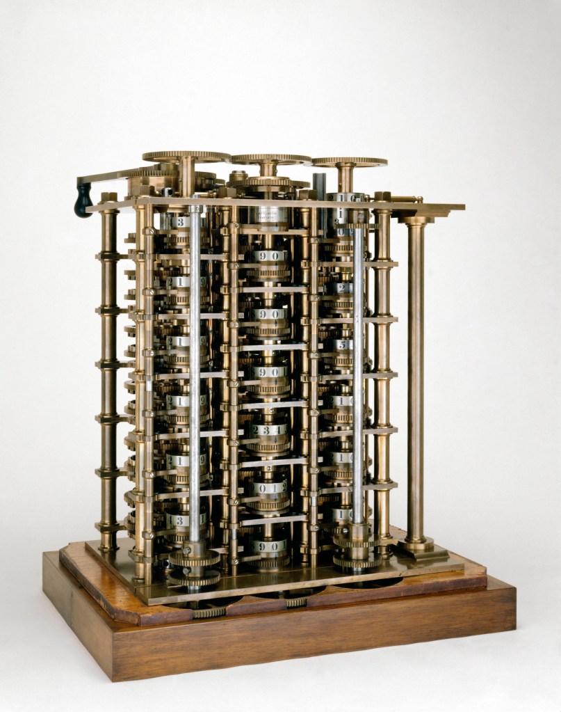
Being unemployed (and unemployable) Babbage had enough time on his hands to actually start work on his engine. He called it the Difference Engine because it worked on the Method of Differences—mathematical formulas were put into a form where a number was expressed as a series, and the differences between each number in the series would be calculated by the engine. He approached the British government for funding, and it obliged with considerable funds. In the days before grant proposals and government funding, Babbage had managed to jump start his project and, in a sense, gain employment. His father was not impressed, but he did not live long enough to see what his son Charles could build. Charles inherited a large sum from his father (the equivalent of about 14 million dollars today), which further freed him to work on his Difference Engine. By 1832, he had finally completed a seventh part of the Engine and displayed it in his house for friends and visitors to see.
This working section of the Difference Engine can be seen today in the London Science Museum. It is a marvel of steel and brass, consisting of three columns of stacked gears whose enmeshed teeth represent digital numbers. As a crank handle is turned, the teath work upon each other, generating new numbers through the permutations of rotated gear teeth. Carrying tens was initially a problem for Babbage, as it is for school children today, but he designed an ingenious mechanical system to accomplish the carry.
All was going well, and the government was pleased with progress, until Charles had a better idea that threatened to scrap all he had achieved. It is not known how this new idea came into being, but it is known that it happened shortly after he met the amazing young woman: Ada Byron.
Lovely Lovelace
Ada Lovelace, born Ada Byron, had the awkward distinction of being the only legitimate child of Lord Byron, lyric genius and poet. Such was Lord Byron’s hedonist lifestyle that no-one can say for sure how many siblings Ada had, not even Lord Byron himself, which was even more awkward when his half-sister bore a bastard child that may have been his.
Fig. 4 Ada Lovelace
Ada’s high-born mother prudently divorced the wayward poet and was not about to have Ada pulled into her father’s morass. Where Lord Byron was bewitched (some would say possessed) by art and spirit, the mother sought an antidote, and she encouraged Ada to study hard cold mathematics. She could not have known that Ada too had a genius like her father’s, only aimed differently, bewitched by the beauty in the sublime symbols of math.
An insight into the precocious child’s way of thinking can be gained from a letter that the 12-year-old girl wrote to her mother who was off looking for miracle cures for imaginary ills. At that time in 1828, in a confluence of historical timelines in the history of mathematics, Ada and her mother (and Ada’s cat Puff) were living at Bifrons House which was the former estate of Brook Taylor, who had developed the Taylor’s series a hundred years earlier in 1715. In Ada’s letter, she describes a dream she had of a flying machine, which is not so remarkable, but then she outlined her plan to her mother to actually make one, which is remarkable. As you read her letter, you see she is already thinking about weights and material strengths and energy efficiencies, thinking like an engineer and designer—at the age of only 12 years!
In later years, Lovelace would become the Enchantress of Number to a number of her mathematical friends, one of whom was the strange man she met at a dinner party in the summer of 1833 when she was 17 years old. The strange man was Charles Babbage, and when he talked to her about his Difference Engine, expecting to be tolerated as an entertaining side show, she asked pertinent questions, one after another, and the two became locked in conversation.
Babbage was a recent widower, having lost his wife with whom he had been happily compatible, and one can only imagine how he felt when the attractive and intelligent woman gave him her attention. But Ada’s mother would never see Charles as a suitable husband for her daughter—she had ambitious plans for her, and she tolerated Babbage only as much as she did because of the affection that Ada had for him. Nonetheless, Ada and Charles became very close as friends and met frequently and wrote long letters to each other, discussing problems and progress on the Difference Engine.
In December of 1834, Charles invited Lady Byron and Ada to his home where he described with great enthusiasm a vision he had of an even greater machine. He called it his Analytical Engine, and it would surpass his Difference Engine in a crucial way: where the Difference Engine needed to be reconfigured by hand before every new calculation, the Analytical Engine would never need to be touched, it just needed to be programmed with punched cards. Charles was in top form as he wove his narrative, and even Lady Byron was caught up in his enthusiasm. The effect on Ada, however, was nothing less than a religious conversion.
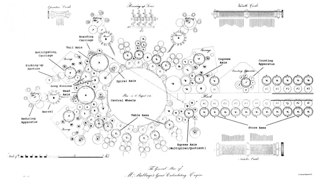
Fig. 5 General block diagram of Babbage’s Analytical Engine. From [8].
Ada’s Notes
To meet Babbage as an equal, Lovelace began to study mathematics with an obsession, or one might say, with delusions of grandeur. She wrote “I believe myself to possess a most singular combination of qualities exactly fitted to make me pre-eminently a discoverer of the hidden realities of nature,” and she was convinced that she was destined to do great things.
Then, in 1835, Ada was married off to a rich but dull aristocrat who was elevated by royal decree to the Earldom of Lovelace, making her the Countess of Lovelace. The marriage had little effect on Charles’ and Ada’s relationship, and he was invited frequently to the new home where they continued their discussions about the Analytical Engine.
By this time Charles had informed the British government that he was putting all his effort into the design his new machine—news that was not received favorably since he had never delivered even a working Difference Engine. Just when he hoped to start work on his Analytical Engine, the government ministers pulled their money. This began a decade’s long ordeal for Babbage as he continued to try to get monetary support as well as professional recognition from his peers for his ideas. Neither attempt was successful at home in Britain, but he did receive interest abroad, especially from a future prime minister of Italy, Luigi Menabrae, who invited Babbage to give a lecture in Turin on his Analytical Engine. Menabrae later had the lecture notes published in French. When Charles Wheatstone, a friend of Babbage, learned of Menabrae’s publication, he suggested to Lovelace that she translate it into English. Menabrae’s publication was the only existing exposition of the Analytical Engine, because Babbage had never written on the Engine himself, and Wheatstone was well aware of Lovelace’s talents, expecting her to be one of the only people in England who had the ability and the connections to Babbage to accomplish the task.
Ada Lovelace dove into the translation of Menabrae’s “Sketch of the Analytical Engine Invented by Charles Babbage” with the single-mindedness that she was known for. Along with the translation, she expanded on the work with Notes of her own that she added, lettered from A to G. By the time she wrote them, Lovelace had become a top-rate mathematician, possibly surpassing even Babbage, and her Notes were three times longer than the translation itself, providing specific technical details and mathematical examples that Babbage and Menabrae only allude to.
On a different level, the character of Ada’s Notes stands in stark contrast to Charles’ exposition as captured by Menabrae: where Menabrae provided only technical details of Babbage’s Engine, Lovelace’s Notes captured the Engine’s potential. She was still a poet by disposition—that inheritance from her father was never lost.
Lovelace wrote:
We may say most aptly, that the Analytical Engine weaves algebraic patterns just as the Jacquard-loom weaves flowers and leaves.
Here she is referring to the punched cards that the Jacquard loom used to program the weaving of intricate patterns into cloth. Babbage had explicitly borrowed this function from Jacquard, adapting it to provide the programmed input to his Analytical Engine.
But it was not all poetics. She also saw the abstract capabilities of the Engine, writing
In studying the action of the Analytical Engine, we find that the peculiar and independent nature of the considerations which in all mathematical analysis belong to operations, as distinguished from the objects operated upon and from the results of the operations performed upon those objects, is very strikingly defined and separated.
Again, it might act upon other things besides number, where objects found whose mutual fundamental relations could be expressed by those of the abstract science of operations, and which should be also susceptible of adaptations to the action of the operating notation and mechanism of the engine.
Supposing, for instance, that the fundamental relations of pitched sounds in the science of harmony and of musical composition were susceptible of such expression and adaptations, the engine might compose elaborate and scientific pieces of music of any degree of complexity or extent.
Here she anticipates computers generating musical scores.
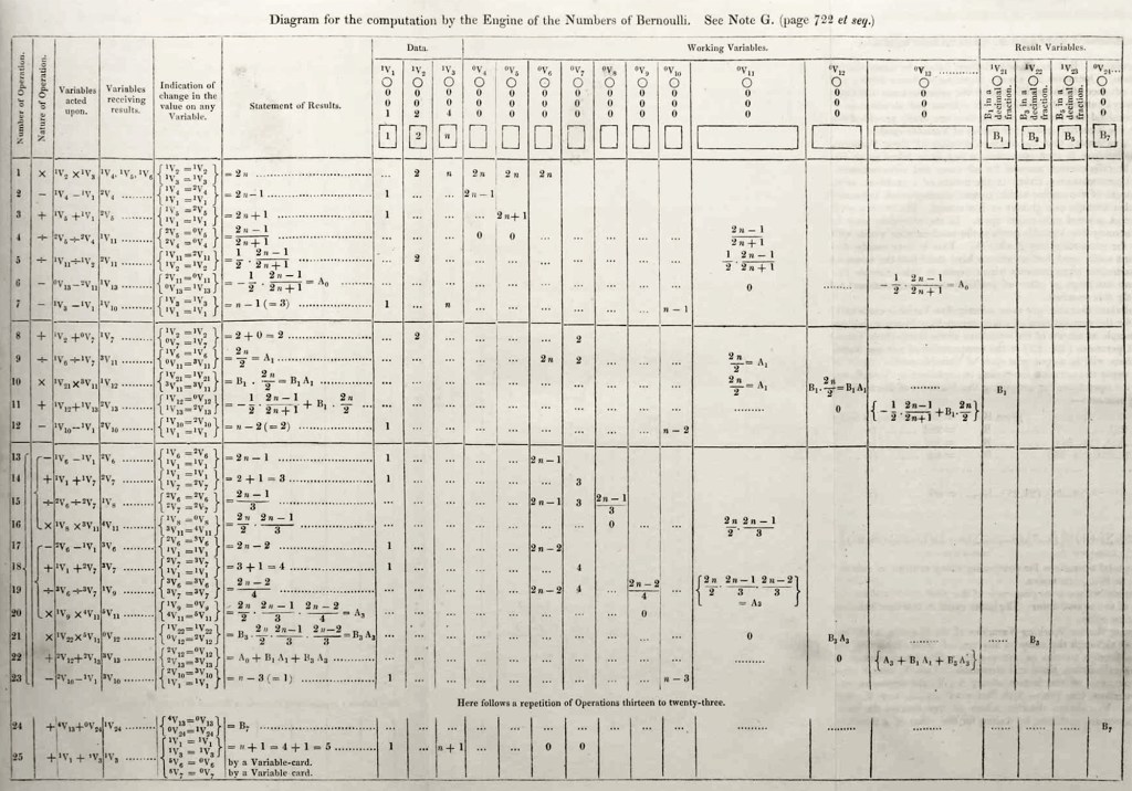
Most striking is Note G. This is where she explicitly describes how the Engine would be used to compute numerical values as solutions to complicated problems. She chose, as her own example, the calculation of Bernoulli numbers which require extensive numerical calculations that were exceptionally challenging even for the best human computers of the day. In Note G, Lovelace writes down the step-by-step process by which the Engine would be programmed by the Jacquard cards to carry out the calculations. In the history of computer science, this stands as the first computer program.
Fig. 6 Table from Lovelace’s Note G on her method to calculate Bernoulli numbers using the Analytical Engine.
When it was time to publish, Babbage read over Lovelace’s notes, checking for accuracy, but he appears to have been uninterested in her speculations, possibly simply glossing over them. He saw his engine as a calculating machine for practical applications. She saw it for what we know today to be the exceptional adaptability of computers to all realms of human study and activity. He did not see what she saw. He was consumed by his Engine to the same degree as she, but where she yearned for the extraordinary, he sought funding for the mundane costs of machining and materials.
Ada’s Business Plan Pitch
Ada Lovelace watched in exasperation as Babbage floundered about with ill-considered proposals to the government while making no real progress towards a working Analytical Engine. Because of her vision into the potential of the Engine, a vision that struck her to her core, and seeing a prime opportunity to satisfy her own yearning to make an indelible mark on the world, she despaired in ever seeing it brought to fruition. Charles, despite his genius, was too impractical, wasting too much time on dead ends and incapable of performing the deft political dances needed to attract support. She, on the other hand, saw the project clearly and had the time and money and the talent, both mathematically and through her social skills, to help.
On Monday August 14, 1843, Ada wrote what might be the most heart-felt and impassioned business proposition in the history of computing. She laid out in clear terms to Charles how she could advance the Analytical Engine to completion if only he would surrender to her the day-to-day authority to make it happen. She was, in essence, proposing to be the Chief Operating Officer in a disruptive business endeavor that would revolutionize thinking machines a hundred years before their time. She wrote (she liked to underline a lot):
“Firstly: I want to know whether if I continue to work on & about your own great subject, you will undertake to abide wholly by the judgment of myself (or of any persons whom you may now please to name as referees, whenever we may differ), on all practical matters relating to whatever can involve relations with any fellow-creature or fellow-creatures.
Secondly: can you undertake to give your mind wholly & undividedly, as a primary object that no engagement is to interfere with, to the consideration of all those matters in which I shall at times require your intellectual assistance & supervision; & can you promise not to slur & hurry things over; or to mislay, & allow confusion and mistakes to enter into documents, &c?
Thirdly: if I am able to lay before you in the course of a year or two, explicit & honorable propositions for executing your engine, (such as are approved by persons whom you may now name to be referred to for their approbation), would there be any chance of your allowing myself & such parties to conduct the business for you; your own undivided energies being devoted to the execution of the work; & all other matters being arranged for you on terms which your own friends should approve?“
This is a remarkable letter from a self-possessed 28-year-old woman, laying out in explicit terms how she proposed to take on the direction of the project, shielding Babbage from the problems of relating to other people or “fellow-creatures” (which was his particular weakness), giving him time to focus his undivided attention on the technical details (which was his particular strength), while she would be the outward face of the project that would attract the appropriate funding.
In her preface to her letter, Ada adroitly acknowledges that she had been a romantic disappointment to Charles, but she pleads with him not to let their personal history cloud his response to her proposal. She also points out that her keen intellect would be an asset to the project and asks that he not dismiss it because of her sex (which a biased Victorian male would likely do). Despite her entreaties, this is exactly what Babbage did. Pencilled on the top of the original version of Ada’s letter in the Babbage archives is his simple note: “Tuesday 15 saw AAL this morning and refused all the conditions”. He had not even given her proposal 24 hours consideration as he indeed slurred and hurried things over.
Aftermath
Babbage never constructed his Analytical Engine and never even wrote anything about it. All his efforts would have been lost to history if Alan Turing had not picked up on Ada’s Notes and expanded upon them a hundred years later, bringing both her and him to the attention of the nascent computing community.
Ada Lovelace died young in 1852, at the age of 36, of cancer. By then she had moved on from Babbage and was working on other things. But she never was able to realize her ambition of uncovering such secrets of nature as to change the world.
Ada had felt from an early age that she was destined for greatness. She never achieved it in her lifetime and one can only wonder what she thought about this as she faced her death. Did she achieve it in posterity? This is a hotly debated question. Some say she wrote the first computer program, which may be true, but little programming a hundred years later derived directly from her work. She did not affect the trajectory of computing history. Discovering her work after the fact is interesting, but cannot be given causal weight in the history of science. The Vikings were the first Europeans to discover America, but no-one knew about it. They did not affect subsequent history the way that Columbus did.
On the other hand, Ada has achieved greatness in a different way. Now that her story is known, she stands as an exemplar of what scientific and technical opportunities look like, and the risk of ignoring them. Babbage also did not achieve greatness during his lifetime, but he could have—if he had not dismissed her and her intellect. He went to his grave embittered rather than lauded because he passed up an opportunity he never recognized.
Mark Twain once famously wrote in a letter from London to a New York newspaper editor:
“I have … heard on good authority that I was dead [but] the report of my death was an exaggeration.”
The same may be true of recent reports on the grave illness and possible impending death of human culture at the hands of ChatGPT and other so-called Large Language Models (LLM). It is argued that these algorithms have such sophisticated access to the bulk of human knowledge, and can write with apparent authority on virtually any topic, that no-one needs to learn or create anything new. It can all be recycled—the end of human culture!
While there may be a kernel of truth to these reports, they are premature. ChatGPT is just the latest in a continuing string of advances that have disrupted human life and human culture ever since the invention of the steam engine. We—humans, that is—weathered the steam engine in the short term and are just as likely to weather the LLM’s.
To start with a very simple example of SLM, imagine you are playing a word scramble game and have the letter “Q”. You can be pretty certain that the “Q“ will be followed by a “U” to make “QU”. Or if you have the initial pair “TH” there is a very high probability that it will be followed by a vowel as “THA…”, “THE…”, ”THI…”, “THO..” or “THU…” and possibly with an “R” as “THR…”. This almost exhausts the probabilities. This is all determined by the statistical properties of English.
Statistical language models build probability distributions for the likelihood that some sequence of letters will be followed by another sequence of letters, or a sequence of words (and punctuations) will be followed by another sequence of words. The bigger the chains of letters and words, the number of possible permutations grows exponentially. This is why SLMs usually stop at some moderate order of statistics. If you build sentences from such a model, it sounds OK for a sentence or two, but then it just drifts around like it’s dreaming or hallucinating in a stream of consciousness without any coherence.
ChatGPT works in much the same way. It just extends the length of the sequences where it sounds coherent up to a paragraph or two. In this sense, it is no more “intelligent” than the SLM that follows “Q” with “U”. ChatGPT simply sustains the charade longer.
Now the details of how ChatGPT accomplishes this charade is nothing less than revolutionary. The acronym GPT means Generative Pre-Trained Transformer. Transformers were a new type of neural net architecture invented in 2017 by the Google Brain team. Transformers removed the need to feed sentences word-by-word into a neural net, instead allowing whole sentences and even whole paragraphs to be input in parallel. Then, by feeding the transformers on more than a Terabyte of textual data from the web, they absorbed the vast output of virtually all the crowd-sourced information from the past 20 years. (This what transformed the model from an SLM to an LLM.) Finally, using humans to provide scores on what good answers looked like versus bad answers, ChatGPT was supervised to provide human-like responses. The result is a chatbot that in any practical sense passes the Turing Test—if you query it for an extended period of time, you would be hard pressed to decide if it was a computer program or a human giving you the answers. But Turing Tests are boring and not very useful.
Figure. The Transformer architecture broken into the training step and the generation step. In training, pairs of inputs and targets are used to train encoders and decoders to build up word probabilities at the output. In generation, a partial input, or a query, is presented to the decoders that find the most likely missing, or next, word in the sequence. The sentence is built up sequentially in each iteration. It is an important distinction that this is not a look-up table … it is trained on huge amounts of data and learns statistical likelihoods, not exact sequences.
The true value of ChatGPT is the access it has to that vast wealth of information (note it is information and not knowledge). Give it almost any moderately technical query, and it will provide a coherent summary for you—on amazingly esoteric topics—because almost every esoteric topic has found its way onto the net by now, and ChatGPT can find it.
As a form of search engine, this is tremendous! Think how frustrating it has always been searching the web for something specific. Furthermore, the lengthened coherence made possible by the transformer neural net means that a first query that leads to an unsatisfactory answer from the chatbot can be refined, and ChatGPT will find a “better” response, conditioned by the statistics of its first response that was not optimal. In a feedback cycle, with the user in the loop, very specific information can be isolated.
Or, imagine that you are not a strong writer, or don’t know the English language as well as you would like. But entering your own text, you can ask ChatGPT to do a copy-edit, even rephrasing your writing where necessary, because ChatGPT above all else has an unequaled command of the structure of English.
Or, for customer service, instead of the frustratingly discrete menu of 5 or 10 potted topics, ChatGPT with a voice synthesizer could respond to continuously finely graded nuances of the customer’s problem—not with any understanding or intelligence, but with probabilistic likelihoods of what the solutions are for a broad range of possible customer problems.
In the midst of all the hype surrounding ChatGPT, it is important to keep in mind two things: First, we are witnessing the beginning of a revolution and a disruptive technology that will change how we live. Second, it is still very early days, just like the early days of the first steam engines running on coal.
Disruptive Technology
Disruptive technologies are the coin of the high-tech realm of Silicon Valley. But this is nothing new. There have always been disruptive technologies—all the way back to Thomas Newcomen and James Watt and the steam engines they developed between 1712 and 1776 in England. At first, steam engines were so crude they were used only to drain water from mines, increasing the number jobs in and around the copper and tin mines of Cornwall (viz. the popular BBC series Poldark) and the coal mines of northern England. But over the next 50 years, steam engines improved, and they became the power source for textile factories that displaced the cottage industry of spinning and weaving that had sustained marginal farms for centuries before.
There is a pattern to a disruptive technology. It not only disrupts an existing economic model, but it displaces human workers. Once-plentiful jobs in an economic sector can vanish quickly after the introduction of the new technology. The change can happen so fast, that there is not enough time for the workforce to adapt, followed by human misery in some sectors. Yet other, newer, sectors always flourish, with new jobs, new opportunities, and new wealth. The displaced workers often never see these benefits because they lack skills for the new jobs.
The same is likely true for the LLMs and the new market models they will launch. There will be a wealth of new jobs curating and editing LLM outputs. There will also be new jobs in the generation of annotated data and in the technical fields surrounding the support of LLMs. LLMs are incredibly hungry for high-quality annotated data in a form best provided by humans. Jobs unlikely to be at risk, despite prophesies of doom, include teachers who can use ChatGPT as an aide by providing appropriate context to its answers. Conversely, jobs that require a human to assemble information will likely disappear, such as news aggregators. The same will be true of jobs in which effort is repeated, or which follow a set of patterns, such as some computer coding jobs or data analysts. Customer service positions will continue to erode, as will library services. Media jobs are at risk, as well as technical writing. The writing of legal briefs may be taken over by LLMs, along with market and financial analysts. By some estimates, there are 300 million jobs around the world that will be impacted one way or another by the coming spectrum of LLMs.
This pattern of disruption is so set and so clear and so consistent, that forward-looking politicians or city and state planners could plan ahead, because we have been on a path of continuing waves disruption for over two hundred years.
Waves of Disruption
In the history of technology, it is common to describe a series of revolutions as if they were distinct. The list looks something like this:
First: Power (The Industrial Revolution: 1760 – 1840)
Second: Electricity and Connectivity (Technological Revolution: 1860 – 1920)
The first revolution revolved around steam power fueled by coal, radically increasing output of goods. The second revolution shifted to electrical technologies, including communication networks through telegraph and the telephones. The third revolution focused on automation and digital information.
Yet this discrete list belies an underlying fact: There is, and has been, only one continuous Industrial Revolution punctuated by waves.
The Age of Industrial Revolutions began around 1760 with the invention of the spinning jenny by James Hargreaves—and that Age has continued, almost without pause, up to today and will go beyond. Each disruptive technology has displaced the last. Each newly trained workforce has been displaced by the last. The waves keep coming.
Note that the fourth wave is happening now, as artificial intelligence matures. This is ironic, because this latest wave of the Industrial Revolution is referred to as the “Imagination Revolution” by the optimists who believe that we are moving into a period where human creativity is unleashed by the unlimited resources of human connectivity across the web. Yet this moment of human ascension to the heights of creativity is happening at just the moment when LLM’s are threatening to remove the need to create anything new.
So is it the end of human culture? Will all knowledge now just be recycled with nothing new added?
A Post-Human Future?
The limitations of the generative aspects of ChatGPT might be best visualized by using an image-based generative algorithm that has also gotten a lot of attention lately. This is the ability to input a photograph, and input a Van Gogh painting, and create a new painting of the photograph in the style of Van Gogh.
In this example, the output on the right looks like a Van Gogh painting. It is even recognizable as a Van Gogh. But in fact it is a parody. Van Gogh consciously created something never before seen by humans.
Even if an algorithm can create “new” art, it is a type of “found” art, like a picturesque stone formation or a sunset. The beauty becomes real only in the response it elicits in the human viewer. Art and beauty do not exist by themselves; they only exist in relationship to the internal state of the conscious observer, like a text or symbol signifying to an interpreter. The interpreter is human, even if the artist is not.
ChatGPT, or any LLM like Google’s Bard, can generate original text, but its value only resides in the human response to it. The human interpreter can actually add value to the LLM text by “finding” sections that are interesting or new, or that inspire new thoughts in the interpreter. The interpreter can also “edit” the text, to bring it in line with their aesthetic values. This way, the LLM becomes a tool for discovery. It cannot “discover” anything on its own, but it can present information to a human interpreter who can mold it into something that they recognize as new. From a semiotic perspective, the LLM can create the signifier, but the signified is only made real by the Human interpreter—emphasize Human.
Therefore, ChatGPT and the LLMs become part of the Fourth Wave of the human Industrial Revolution rather than replacing it.
We are moving into an exciting time in the history of technology, giving us a rare opportunity to watch as the newest wave of revolution takes shape before our very eyes. That said … just as the long-term consequences of the steam engine are only now coming home to roost two hundred years later in the form of threats to our global climate, the effect of ChatGPT in the long run may be hard to divine until far in the future—and then, maybe after it’s too late, so a little caution now would be prudent.
Physics forged ahead in 2022, making a wide range of advances. From a telescope far out in space to a telescope that spans the size of the Earth, from solid state physics and quantum computing at ultra-low temperatures to particle and nuclear physics at ultra-high energies, the year saw a number of firsts. Here’s a list of eight discoveries of 2022 that define the frontiers of physics.
James Webb Space Telescope
“First Light” has two meanings: the “First Light” that originated at the beginning of the universe, and the “First Light” that is collected by a new telescope. In the beginning of this year, the the James Webb Space Telescope (JWST) saw both types of first light, and with it came first surprises.
NASA image of the Carina Nebula, a nursery for stars.
The JWST has found that galaxies are too well formed too early in the universe relative to current models of galaxy formation. Almost as soon as the JWST began forming images, it acquired evidence of massive galaxies from only a few hundred million years old. Existing theories of galaxy formation did not predict such large galaxies so soon after the Big Bang.
Another surprise came from images of the Southern Ring Nebula. While the Hubble did not find anything unusual about this planetary nebula, the JWST found cold dust surrounding the white dwarf that remained after the explosion of the supernova. This dust was not supposed to be there, but it may be coming from a third member of the intra-nebular environment. In addition, the ring-shaped nebula contained masses of swirling streams and ripples that are challenging astrophysicists who study supernova and nebula formation to refine their current models.
Quantum Machine Learning
Machine learning—the training of computers to identify and manipulate complicated patterns within massive data—has been on a roll in recent years, ever since efficient training algorithms were developed in the early 2000’s for large multilayer neural networks. Classical machine learning can take billions of bits of data and condense it down to understandable information in a matter of minutes. However, there are types of problems that even conventional machine learning might take the age of the universe to calculate, for instance calculating the properties of quantum systems based on a set of quantum measurements of the system.
In June of 2022, researchers at Caltech and Google announced that a quantum computer—Google’s Sycamore quantum computer—could calculate properties of quantum systems using exponentially fewer measurements than would be required to perform the same task using conventional computers. Quantum machine learning uses the resource of quantum entanglement that is not available to conventional machine learning, enabling new types of algorithms that can exponentially speed up calculations of quantum systems. It may come as no surprise that quantum computers are ideally suited to making calculations of quantum systems.
Science News. External view of Google’s Sycamore quantum computer.
A Possible Heavy W Boson
High-energy particle physics has been in a crisis ever since 2012 when they reached the pinnacle of a dogged half-century search for the fundamental constituents of the universe. The Higgs boson was the crowning achievement, and was supposed to be the vanguard of a new frontier of physics uncovered by CERN. But little new physics has emerged, even though fundamental physics is in dire need of new results. For instance, dark matter and dark energy remain unsolved mysteries despite making up the vast majority of all there is. Therefore, when physicists at Fermilab announced that the W boson, a particle that carries the nuclear weak interaction, was heavier than predicted by the Standard Model, some physicists heaved sighs of relief. The excess mass could signal higher-energy contributions that might lead to new particles or interactions … if the excess weight holds up under continued scrutiny.
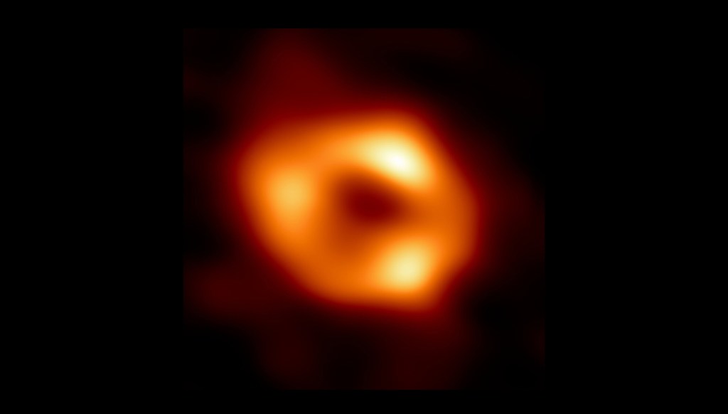
Imaging the Black Hole at the Center of the Milky Way
Imagine building a telescope the size of the Earth. What could it see?
If it detected in the optical regime, it could see a baseball on the surface of the Moon. If it detected at microwave frequencies, then it could see the material swirling around distant black holes. This is what the Event Horizon Telescope (EHT) can do. In 2019, it revealed the first image of a black hole: the super-massive black hole at the core of the M87 galaxy 53 million light years away. They did this Herculean feat by combining the signals of microwave telescopes from across the globe, combining their signals interferometrically to create an effective telescope aperture that was the size of the Earth.
The next obvious candidate was the black hole at the center of our own galaxy, the Milky Way. Even though our own black hole is much smaller than the one in M87, ours is much closer, and both subtend about the same solid angle. The challenge was observing it through the swirling stars and dust at the core of our galaxy. In May of this year, the EHT unveiled the first image of our own black hole, showing the radiation emitted by the in-falling material.
BBC image of the black hole at the core of our Milky Way galaxy.
Tetraneutrons
Nuclear physics is a venerable part of modern physics that harkens back to the days of Bohr and Rutherford and the beginning of quantum physics, but in recent years it has yielded few new surprises (except at the RHIC collider which smashes heavy nuclei against each other to create quark-gluon plasma). That changed in June of 2022, when researchers in Germany announced the successful measurement of a tetraneutron–a cluster of four neutrons bound transiently together by the strong nuclear force.
Neutrons are the super-glue that holds together the nucleons in standard nuclei. The force is immense, strong enough to counteract the Coulomb repulsion of protons in a nucleus. For instance, Uranium 238 has 92 protons crammed within a volume of about 10 femtometer radius. It takes 146 neutrons to bind these together without flying apart. But neutrons don’t tend to bind to themselves, except in “resonance” states that decay rapidly. In 2012, a dineutron (two neutrons bound in a transient resonance state) was observed, but four neutrons were expected to produce an even more transient resonance (a three-neutron state is not allowed). When the German group created the tetraneutron, it had a lifetime of only about 1×10-21 seconds, so it is extremely ephemeral. Nonetheless, studying the properties of the tetraneutron may give insights into both the strong and weak nuclear forces.
Hi-Tc superconductivity
When Bednorz and Müller discovered Hi-Tc superconductivity in 1986, it set off both a boom and a crisis. The boom was the opportunity to raise the critical temperature of superconductivity from 23 K that had been the world record held by Nb3Ge for 13 years since it was set in 1973. The crisis was that the new Hi-Tc materials violated the established theory of superconductivity explained by Bardeen-Cooper-Schrieffer (BCS). There was almost nothing in the theory of solid state physics that could explain how such high critical temperatures could be attained. At the March Meeting of the APS the following year in 1987, the session on the new Hi-Tc materials and possible new theories became known as the Woodstock of Physics, where physicists camped out in the hallway straining their ears to hear the latest ideas on the subject.
One of the ideas put forward at the session was the idea of superexchange by Phil Anderson. The superexchange of two electrons is related to their ability to hop from one lattice site to another. If the hops are coordinated, then there can be an overall reduction in their energy, creating a ground state of long-range coordinated electron hopping that could support superconductivity. Anderson was perhaps the physicist best situated to suggest this theory because of his close familiarity with what was, even then, known as the Anderson Hamiltonian that explicitly describes the role of hopping in solid-state many-body phenomena.
Ever since, the idea of superexchange has been floating around the field of Hi-Tc superconductivity, but no one had been able to pin it down conclusively, until now. In a paper published in the PNAS in September of 2022, an experimental group at Oxford presented direct observations of the spatial density of Cooper pairs in relation to the spatial hopping rates—where hopping was easiest then the Cooper pair density was highest, and vice versa. This experiment provides almost indisputable evidence in favor of Anderson’s superexchange mechanism for Cooper pair formation in the Hi-Tc materials, laying to rest the crisis launched 36 years ago.
Holographic Wormhole
The holographic principle of cosmology proposes that our three-dimensional physical reality—stars, galaxies, expanding universe—is like the projection of information encoded on a two-dimensional boundary—just as a two-dimensional optical hologram can be illuminated to recreate a three-dimensional visual representation. This 2D to 3D projection was first proposed by Gerald t’Hooft, inspired by the black hole information paradox in which the entropy of a black hole scales as surface area of the black hole instead of its volume. The holographic principle was expanded by Leonard Susskind in 1995 based on string theory and is one path to reconciling quantum physics with the physics of gravitation in a theory of quantum gravity—one of the Holy Grails of physics.
While it is an elegant cosmic idea, the holographic principle could not be viewed as anything down to Earth, until now. In November 2022 a research group at Caltech published a paper in Nature describing how they used Google’s Sycamore quantum computer (housed at UC Santa Barbara) to manipulate a set of qubits into creating a laboratory-based analog of a Einstein-Rosen bridge, also known as a “wormhole”, through spacetime. The ability to use quantum information states to simulate a highly-warped spacetime analog provides the first experimental evidence for the validity of the cosmological holographic principle. Although the simulation did not produce a physical wormhole in our spacetime, it showed how quantum information and differential geometry (the mathematics of general relativity) can be connected.
One of the most important consequences of this work is the proposal that ER = EPR (Einstein-Rosen = Einstein-Podolsky-Rosen). The EPR paradox of quantum entanglement has long been viewed as a fundamental paradox of physics that requires instantaneous non-local correlations among quantum particles that can be arbitrarily far apart. Although EPR violates local realism, it is a valuable real-world resource for quantum teleportation. By demonstrating the holographic wormhole, the recent Caltech results show how quantum teleportation and gravitational wormholes may arise from the same physics.
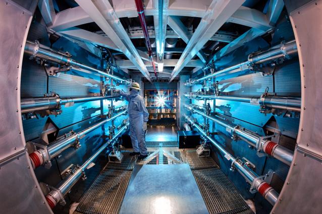
Net-Positive-Energy from Nuclear Fusion
Ever since nuclear fission was harnessed to generate energy, the idea of tapping the even greater potential of nuclear fusion to power the world has been a dream of nuclear physicists. Nuclear fusion energy would be clean and green and could help us avoid the long-run disaster of global warming. However, achieving that dream has been surprisingly frustrating. While nuclear fission was harnessed for energy (and weapons) within only a few years of discovery, and a fusion “boost” was added to nuclear destructive power in the so-called hydrogen bomb, sustained energy production from fusion has remained elusive.
In December of 2022, the National Ignition Facility (NIF) focussed the power of 192 pulsed lasers onto a deuterium-tritium pellet, causing it to implode, and the nuclei to fuse, releasing about 50% more energy that it absorbed. This was the first time that controlled fusion released net positive energy—about 3 million Joules out from 2 million Joules in—enough energy to boil about 3 liters of water. This accomplishment represents a major milestone in the history of physics and could one day provide useful energy. The annual budget of the NIF is about 300 million dollars, so there is a long road ahead (probably several more decades) before this energy source can be scaled down to an economical level.
When our son was ten years old, he came home from a town fair in Battleground, Indiana, with an unwanted pet—a goldfish in a plastic bag. The family rushed out to buy a fish bowl and food and plopped the golden-red animal into it. In three days, it was dead!
It turns out that you can’t just put a gold fish in a fish bowl. When it metabolizes its food and expels its waste, it builds up toxic levels of ammonia unless you add filters or plants or treat the water with chemicals. In the end, the goldfish died because it was asphyxiated by its own pee.
It’s a basic rule—don’t pee in your own fish bowl.
The same can be said for humans living on the surface of our planet. Polluting the atmosphere with our wastes cannot be a good idea. In the end it will kill us. The atmosphere may look vast—the fish bowl was a big one—but it is shocking how thin it is.
Turn on your Apple TV, click on the screen saver, and you are skimming over our planet on the dark side of the Earth. Then you see a thin blue line extending over the limb of the dark disc. Hold! That thin blue line! That is our atmosphere! Is it really so thin?
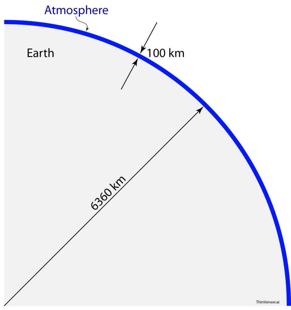
When you look upwards on a clear sunny day, the atmosphere seems like it goes on forever. It doesn’t. It is a thin veneer on the surface of the Earth barely one percent of the Earth’s radius. The Earth’s atmosphere is frighteningly thin.
Fig. 1 A thin veneer of atmosphere paints the surface of the Earth. The radius of the Earth is 6360 km, and the thickness of the atmosphere is 100 km, which is a bit above 1 percent of the radius.
Consider Mars. It’s half the size of Earth, yet it cannot hold on to an atmosphere even 1/100th the thickness of ours. When Mars first formed, it had an atmosphere not unlike our own, but through the eons its atmosphere has wafted away irretrievably into space.
An atmosphere is a precious fragile thing for a planet. It gives life and it gives protection. It separates us from the deathly cold of space, holding heat like a blanket. That heat has served us well over the eons, allowing water to stay liquid and allowing life to arise on Earth. But too much of a good thing is not a good thing.
Common Sense
If the fluid you are bathed in gives you life, then don’t mess with it. Don’t run your car in the garage while you are working in it. Don’t use a charcoal stove in an enclosed space. Don’t dump carbon dioxide into the atmosphere because it alsois an enclosed space.
At the end of winter, as the warm spring days get warmer, you take the winter blanket off your bed because blankets hold in heat. The thicker the blanket, the more heat it holds in. Common sense tells you to reduce the thickness of the blanket if you don’t want to get too warm. Carbon dioxide in the atmosphere acts like a blanket. If we don’t want the Earth to get too warm, then we need to limit the thickness of the blanket.
Without getting into the details of any climate change model, common sense already tells us what we should do. Keep the atmosphere clean and stable (Don’t’ pee in our fishbowl) and limit the amount of carbon dioxide we put into it (Don’t let the blanket get too thick).
Some Atmospheric Facts
Here are some facts about the atmosphere, about the effect humans have on it, and about the climate:
Fact 1. Humans have increased the amount of carbon dioxide in the atmosphere by 45% since 1850 (the beginning of the industrial age) and by 30% since just 1960.
Fact 2. Carbon dioxide in the atmosphere prevents some of the heat absorbed from the Sun to re-radiate out to space. More carbon dioxide stores more heat.
Fact 3. Heat added to the Earth’s atmosphere increases its temperature. This is a law of physics.
Fact 4. The Earth’s average temperature has risen by 1.2 degrees Celsius since 1850 and 0.8 degrees of that has been just since 1960, so the effect is accelerating.
These facts are indisputable. They hold true regardless of whether there is a Republican or a Democrat in the White House or in control of Congress.
There is another interesting observation which is not so direct, but may hold a harbinger for the distant future: The last time the Earth was 3 degrees Celsius warmer than it is today was during the Pliocene when the sea level was tens of meters higher. If that sea level were to occur today, all of Delaware, most of Florida, half of Louisiana and the entire east coast of the US would be under water, including Houston, Miami, New Orleans, Philadelphia and New York City. There are many reasons why this may not be an immediate worry. The distribution of water and ice now is different than in the Pliocene, and the effect of warming on the ice sheets and water levels could take centuries. Within this century, the amount of sea level rise is likely to be only about 1 meter, but accelerating after that.
Fig. 2 The east coast of the USA for a sea level 30 meters higher than today. All of Delaware, half of Louisiana, and most of Florida are under water. Reasonable projections show only a 1 meter sea level rise by 2100, but accelerating after that. From https://www.youtube.com/watch?v=G2x1bonLJFA
Balance and Feedback
It is relatively easy to create a “rule-of-thumb” model for the Earth’s climate (see Ref. [2]). This model is not accurate, but it qualitatively captures the basic effects of climate change and is a good way to get an intuitive feeling for how the Earth responds to changes, like changes in CO2 or to the amount of ice cover. It can also provide semi-quantitative results, so that relative importance of various processes or perturbations can be understood.
The model is a simple energy balance statement: In equilibrium, as much energy flows into the Earth system as out.
This statement is both simple and immediately understandable. But then the work starts as we need to pin down how much energy is flowing in and how much is flowing out. The energy flowing in comes from the sun, and the energy flowing out comes from thermal radiation into space.
We also need to separate the Earth system into two components: the surface and the atmosphere. These are two very different things that have two different average temperatures. In addition, the atmosphere transmits sunlight to the surface, unless clouds reflect it back into space. And the Earth radiates thermally into space, unless clouds or carbon dioxide layers reflect it back to the surface.
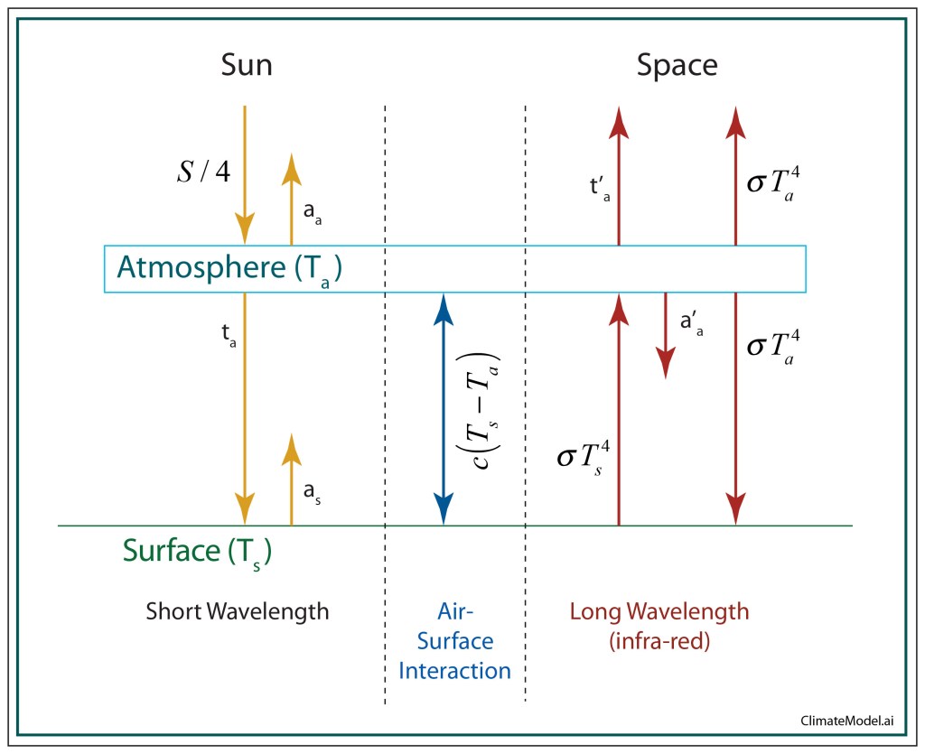
The energy fluxes are shown in the diagram in Fig. 3 for the 4-component system: Sun, Surface, Atmosphere, and Space. The light from the sun, mostly in the visible range of the spectrum, is partially absorbed by the atmosphere and partially transmitted and reflected. The transmitted portion is partially absorbed and partially reflected by the surface. The heat of the Earth is radiated at long wavelengths to the atmosphere, where it is partially transmitted out into space, but also partially reflected by the fraction a’a which is the blanket effect. In addition, the atmosphere itself radiates in equal parts to the surface and into outer space. On top of all of these radiative processes, there is also non-radiative convective interaction between the atmosphere and the surface.
Fig. 3 Energy flux model for a simple climate model with four interacting systems: the Sun, the Atmosphere, the Earth and Outer Space.
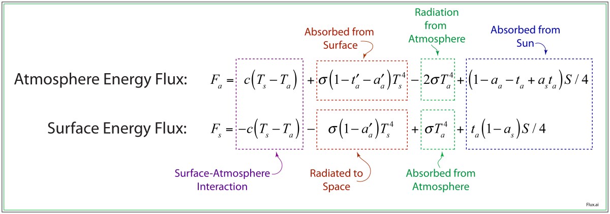
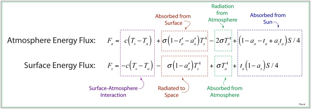
These processes are captured by two energy flux equations, one for the atmosphere and one for the surface, in Fig. 4. The individual contributions from Fig. 3 are annotated in each case. In equilibrium, each flux equals zero, which can then be used to solve for the two unknowns: Ts0 and Ta0: the surface and atmosphere temperatures.
Fig. 4 Energy-balance model of the Earth’s atmosphere for a simple climate approximation.
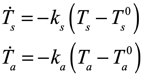
After the equilibrium temperatures Ts0 and Ta0 are found, they go into a set of dynamic response equations that governs how deviations in the temperatures relax back to the equilibrium values. These relaxation equations are
where ks and ka are the relaxation rates for the surface and atmosphere. These can be quite slow, in the range of a century. For illustration, we can take ks = 1/75 years and ka = 1/25 years. The equilibrium temperatures for the surface and atmosphere differ by about 50 degrees Celsius, with Ts = 289 K and Ta = 248 K. These are rough averages over the entire planet. The solar constant is S = 1.36×10³ W/m2, the Stefan-Boltzman constant is σ = 5.67×10⁻⁸ W/m2/K4, and the convective interaction constant is c = 2.5 W m-2 K-1. Other parameters are given in Table I.
Short Wavelength
Long Wavelength
as = 0.11
ts = 0.53
t’a = 0.06
aa = 0.30
a’a = 0.31
The relaxation equations are in the standard form of a mathematical “flow” (see Ref. [1]) and the solutions are plotted as a phase-space portrait in Fig. 5 as a video of the flow as the parameters in Table I shift because of the addition of greenhouse gases to the atmosphere. The video runs from the year 1850 (the dawn of the industrial age) through to the year 2060 about 40 years from now.
Fig. 5 Video of the phase space flow of the Surface-Atmosphere system for increasing year. The flow vectors and flow lines are the relaxation to equilibrium for temperature deviations. The change in equilibrium over the years is from increasing blanket effects in the atmosphere caused by greenhouse gases.
The scariest part of the video is how fast it accelerates. From 1850 to 1950 there is almost no change, but then it accelerates, faster and faster, reflecting the time-lag in temperature rise in response to increased greenhouse gases.
What if the Models are Wrong? Russian Roulette
Now come the caveats.
This model is just for teaching purposes, not for any realistic modeling of climate change. It captures the basic physics, and it provides a semi-quantitative set of parameters that leads to roughly accurate current temperatures. But of course, the biggest elephant in the room is that it averages over the entire planet, which is a very crude approximation.
It does get the basic facts correct, though, showing an alarming trend in the rise in average temperatures with the temperature rising by 3 degrees by 2060.
The professionals in this business have computer models that are orders of magnitude more more accurate than this one. To understand the details of the real climate models, one needs to go to appropriate resources, like this NOAA link, this NASA link, this national climate assessment link, and this government portal link, among many others.
One of the frequent questions that is asked is: What if these models are wrong? What if global warming isn’t as bad as these models say? The answer is simple: If they are wrong, then the worst case is that life goes on. If they are right, then in the worst case life on this planet may end.
It’s like playing Russian Roulette. If just one of the cylinders on the revolver has a live bullet, do you want to pull the trigger?
Matlab Code
function flowatmos.m

mov_flag = 1;
if mov_flag == 1
    moviename = 'atmostmp';
    aviobj = VideoWriter(moviename,'MPEG-4');
    aviobj.FrameRate = 12;
    open(aviobj);
end

Solar = 1.36e3;		% Solar constant outside atmosphere [J/sec/m2]
sig = 5.67e-8;		% Stefan-Boltzman constant [W/m2/K4]

% 1st-order model of Earth + Atmosphere

ta = 0.53;			% (0.53)transmissivity of air
tpa0 = 0.06;			% (0.06)primes are for thermal radiation
as0 = 0.11;			% (0.11)
aa0 = 0.30;			% (0.30)
apa0 = 0.31;        % (0.31)
c = 2.5;               % W/m2/K

xrange = [287 293];
yrange = [247 251];

rngx = xrange(2) - xrange(1);
rngy = yrange(2) - yrange(1);

[X,Y] = meshgrid(xrange(1):0.05:xrange(2), yrange(1):0.05:yrange(2));

smallarrow = 1;
Delta0 = 0.0000009;
for tloop =1:80

    Delta = Delta0*(exp((tloop-1)/8)-1);   % This Delta is exponential, but should become more linear over time
    date = floor(1850 + (tloop-1)*(2060-1850)/79);

    [x,y] = f5(X,Y);

    clf
    hold off
    eps = 0.002;
    for xloop = 1:11
        xs = xrange(1) +(xloop-1)*rngx/10 + eps;
        for yloop = 1:11
            ys = yrange(1) +(yloop-1)*rngy/10 + eps;

            streamline(X,Y,x,y,xs,ys)

        end
    end
    hold on
    [XQ,YQ] = meshgrid(xrange(1):1:xrange(2),yrange(1):1:yrange(2));
    smallarrow = 1;
    [xq,yq] = f5(XQ,YQ);
    quiver(XQ,YQ,xq,yq,.2,'r','filled')
    hold off

    axis([xrange(1) xrange(2) yrange(1) yrange(2)])
    set(gcf,'Color','White')

    fun = @root2d;
    x0 = [0 -40];
    x = fsolve(fun,x0);

    Ts = x(1) + 288
    Ta = x(2) + 288

    hold on
    rectangle('Position',[Ts-0.05 Ta-0.05 0.1 0.1],'Curvature',[1 1],'FaceColor',[1 0 0],'EdgeColor','k','LineWidth',2)

    posTs(tloop) = Ts;
    posTa(tloop) = Ta;

    plot(posTs,posTa,'k','LineWidth',2);
    hold off

    text(287.5,250.5,strcat('Date = ',num2str(date)),'FontSize',24)
    box on
    xlabel('Surface Temperature (oC)','FontSize',24)
    ylabel('Atmosphere Temperature (oC)','FontSize',24)

    hh = figure(1);
    pause(0.01)
    if mov_flag == 1
        frame = getframe(hh);
        writeVideo(aviobj,frame);
    end

end     % end tloop

if mov_flag == 1
    close(aviobj);
end

    function F = root2d(xp)   % Energy fluxes

        x = xp + 288;
        feedfac = 0.001;      % feedback parameter

        apa = apa0 + feedfac*(x(2)-248) + Delta;  % Changes in the atmospheric blanket
        tpa = tpa0 - feedfac*(x(2)-248) - Delta;
        as = as0 - feedfac*(x(1)-289);

        F(1) = c*(x(1)-x(2)) + sig*(1-apa)*x(1).^4 - sig*x(2).^4 - ta*(1-as)*Solar/4;
        F(2) = c*(x(1)-x(2)) + sig*(1-tpa - apa)*x(1).^4 - 2*sig*x(2).^4 + (1-aa0-ta+as*ta)*Solar/4;

    end

    function [x,y] = f5(X,Y)   % Dynamical flow equations

        k1 = 1/75;   % 75 year time constant for the Earth
        k2 = 1/25;   % 25 year time constant for the Atmosphere

        fun = @root2d;
        x0 = [0 0];
        x = fsolve(fun,x0);   % Solve for the temperatures that set the energy fluxes to zero

        Ts0 = x(1) + 288;   % Surface temperature in Kelvin
        Ta0 = x(2) + 288;   % Atmosphere temperature in Kelvin

        xtmp = -k1*(X - Ts0);   % Dynamical equations
        ytmp = -k2*(Y - Ta0);

        nrm = sqrt(xtmp.^2 + ytmp.^2);

        if smallarrow == 1
            x = xtmp./nrm;
            y = ytmp./nrm;
        else
            x = xtmp;
            y = ytmp;
        end

    end     % end f5

end       % end flowatmos
This model has a lot of parameters that can be tweaked. In addition to the parameters in the Table, the time dependence on the blanket properties of the atmosphere are governed by Delta0 and by feedfac for feedback of temperature on the atmosphere, such as increasing cloud cover and decrease ice cover. As an exercise, and using only small changes in the given parameters, find the following cases: 1) An increasing surface temperature is moderated by a falling atmosphere temperature; 2) The Earth goes into thermal run-away and ends like Venus; 3) The Earth initially warms then plummets into an ice age.
The ability to travel to the stars has been one of mankind’s deepest desires. Ever since we learned that we are just one world in a vast universe of limitless worlds, we have yearned to visit some of those others. Yet nature has thrown up an almost insurmountable barrier to that desire–the speed of light. Only by traveling at or near the speed of light may we venture to far-off worlds, and even then, decades or centuries will pass during the voyage. The vast distances of space keep all the worlds isolated–possibly for the better.
Yet the closest worlds are not so far away that they will always remain out of reach. The very limit of the speed of light provides ways of getting there within human lifetimes. The non-intuitive effects of special relativity come to our rescue, and we may yet travel to the closest exoplanet we know of.
Proxima Centauri b
The closest habitable Earth-like exoplanet is Proxima Centauri b, orbiting the red dwarf star Proxima Centauri that is about 4.2 lightyears away from Earth. The planet has a short orbital period of only about 11 Earth days, but the dimness of the red dwarf puts the planet in what may be a habitable zone where water is in liquid form. Its official discovery date was August 24, 2016 by the European Southern Observatory in the Atacama Desert of Chile using the Doppler method. The Alpha Centauri system is a three-star system, and even before the discovery of the planet, this nearest star system to Earth was the inspiration for the Hugo-Award winning sci-fi trilogy The Three Body Problem by Chinese author Liu Cixin, originally published in 2008.
It may seem like a coincidence that the closest Earth-like planet to Earth is in the closest star system to Earth, but it says something about how common such exoplanets may be in our galaxy.
Artist’s rendition of Proxima Centauri b. From WikiCommons.
Breakthrough Starshot
There are already plans to send centimeter-sized spacecraft to Alpha Centauri. One such project that has received a lot of press is Breakthrough Starshot, a project of the Breakthrough Initiatives. Breakthrough Starshot would send around 1000 centimeter-sized camera-carrying laser-fitted spacecraft with 5-meter-diameter solar sails propelled by a large array of high-power lasers. The reason there are so many of these tine spacecraft is because of the collisions that are expected to take place with interstellar dust during the voyage. It is possible that only a few dozen of the craft will finally make it to Alpha Centauri intact.
Relative locations of the stars of the Alpha Centauri system. From ScienceNews.
As these spacecraft fly by the Alpha Centauri system, possibly within one hundred million miles of Proxima Centauri b, their tiny HR digital cameras will take pictures of the planet’s surface with enough resolution to see surface features. The on-board lasers will then transmit the pictures back to Earth. The travel time to the planet is expected to be 20 or 30 years, plus the four years for the laser information to make it back to Earth. Therefore, it would take a quarter century after launch to find out if Proxima Centauri b is habitable or not. The biggest question is whether it has an atmosphere. The red dwarf it orbits sends out catastrophic electromagnetic bursts that could strip the planet of its atmosphere thus preventing any chance for life to evolve or even to be sustained there if introduced.
There are multiple projects under consideration for travel to the Alpha Centauri systems. Even NASA has a tentative mission plan called the 2069 Mission (100 year anniversary of the Moon landing). This would entail a single spacecraft with a much larger solar sail than the small starshot units. Some of the mission plans proposed star-drive technology, such as nuclear propulsion systems, rather than light sails. Some of these designs could sustain a 1-g acceleration throughout the entire mission. It is intriguing to do the math on what such a mission could look like, in terms of travel time. Could we get an unmanned probe to Alpha Centauri in a matter of years? Let’s find out.
Special Relativity of Acceleration
The most surprising aspect of deriving the properties of relativistic acceleration using special relativity is that it works at all. We were all taught as young physicists that special relativity deals with inertial frames in constant motion. So the idea of frames that are accelerating might first seem to be outside the scope of special relativity. But one of Einstein’s key insights, as he sought to extend special relativity towards a more general theory, was that one can define a series of instantaneously inertial co-moving frames relative to an accelerating body. In other words, at any instant in time, the accelerating frame has an inertial co-moving frame. Once this is defined, one can construct invariants, just as in usual special relativity. And these invariants unlock the full mathematical structure of accelerating objects within the scope of special relativity.
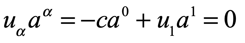
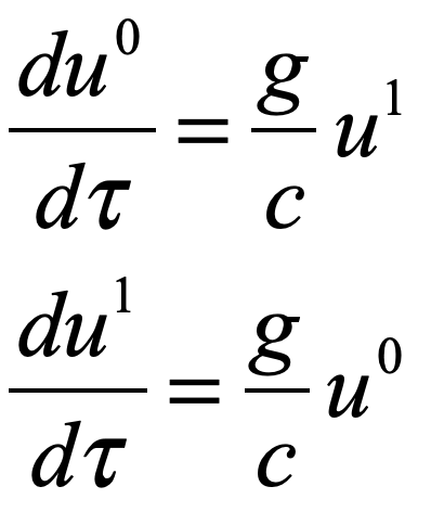
For instance, the four-velocity and the four-acceleration in a co-moving frame for an object accelerating at g are given by
The object is momentarily stationary in the co-moving frame, which is why the four-velocity has only the zeroth component, and the four-acceleration has simply g for its first component.
Armed with these four-vectors, one constructs the invariants
and
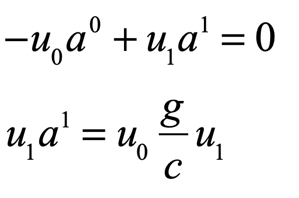
This last equation is solved for the specific co-moving frame as
But the invariant is more general, allowing the expression
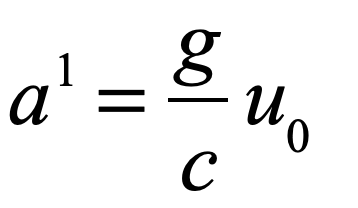
which yields
From these, putting them all together, one obtains the general differential equations for the change in velocity as a set of coupled equations
The solution to these equations is
where the unprimed frame is the lab frame (or Earth frame), and the primed frame is the frame of the accelerating object, for instance a starship heading towards Alpha Centauri. These equations allow one to calculate distances, times and speeds as seen in the Earth frame as well as the distances, times and speeds as seen in the starship frame. If the starship is accelerating at some acceleration g’ other than g, then the results are obtained simply by replacing g by g’ in the equations.
Relativistic Flight
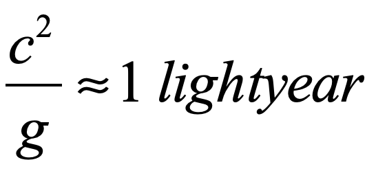
It turns out that the acceleration due to gravity on our home planet provides a very convenient (but purely coincidental) correspondence
With a similarly convenient expression
These considerably simplify the math for a starship accelerating at g.
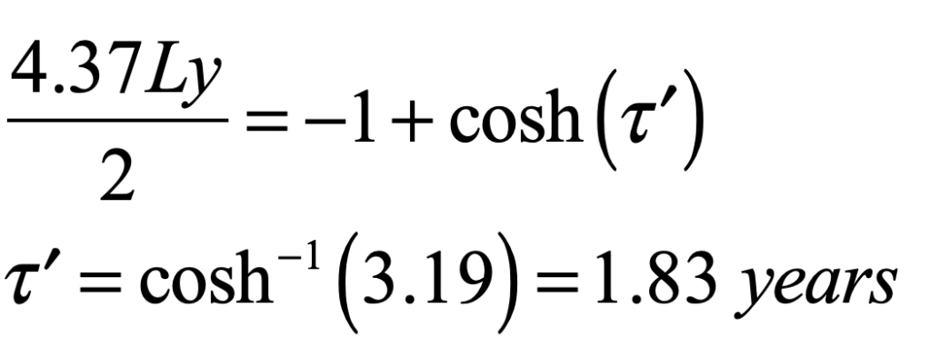
Let’s now consider a starship accelerating by g for the first half of the flight to Alpha Centauri, turning around and decelerating at g for the second half of the flight, so that the starship comes to a stop at its destination. The equations for the times to the half-way point are
This means at the midpoint that 1.83 years have elapsed on the starship, and about 3 years have elapsed on Earth. The total time to get to Alpha Centauri (and come to a stop) is then simply
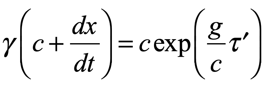
It is interesting to look at the speed at the midpoint. This is obtained by
which is solved to give
This amazing result shows that the starship is traveling at 95% of the speed of light at the midpoint when accelerating at the modest value of g for about 3 years. Of course, the engineering challenges for providing such an acceleration for such a long time are currently prohibitive … but who knows? There is a lot of time ahead of us for technology to advance to such a point in the next century or so.
Figure. Time lapsed inside the spacecraft and on Earth for the probe to reach Alpha Centauri as a function of the acceleration of the craft. At 10 g’s, the time elapsed on Earth is a little less than 5 years. However, the signal sent back will take an additional 4.37 years to arrive for a total time of about 9 years.
Matlab alphacentaur.m
% alphacentaur.m
clear
format compact

g0 = 1;
L = 4.37;

for loop = 1:100

    g = 0.1*loop*g0;

    taup = (1/g)*acosh(g*L/2 + 1);
    tearth = (1/g)*sinh(g*taup);

    tauspacecraft(loop) = 2*taup;
    tlab(loop) = 2*tearth;

    acc(loop) = g;

end

figure(1)
loglog(acc,tauspacecraft,acc,tlab,'LineWidth',2)
legend('Space Craft','Earth Frame','FontSize',18)
xlabel('Acceleration (g)','FontSize',18)
ylabel('Time (years)','FontSize',18)
dum = set(gcf,'Color','White');
H = gca;
H.LineWidth = 2;
H.FontSize = 18;
To Centauri and Beyond
Once we get unmanned probes to Alpha Centauri, it opens the door to star systems beyond. The next closest are Barnards star at 6 Ly away, Luhman 16 at 6.5 Ly, Wise at 7.4 Ly, and Wolf 359 at 7.9 Ly. Several of these are known to have orbiting exoplanets. Ross 128 at 11 Ly and Lyuten at 12.2 Ly have known earth-like planets. There are about 40 known earth-like planets within 40 lightyears from Earth, and likely there are more we haven’t found yet. It is almost inconceivable that none of these would have some kind of life. Finding life beyond our solar system would be a monumental milestone in the history of science. Perhaps that day will come within this century.
This Blog Post is a Companion to the undergraduate physics textbook Modern Dynamics: Chaos, Networks, Space and Time, 2nd ed. (Oxford, 2019) introducing Lagrangians and Hamiltonians, chaos theory, complex systems, synchronization, neural networks, econophysics and Special and General Relativity.
An old joke goes that Democracy is a terrible form of government … except it’s better than all the others!
Our world today is faced with conflict between democracy and dictatorship. On the one side is the free world, where leaders are chosen by some form of representation of large numbers of citizens and sometimes even a majority. On the other side is authoritarianism where a select few are selected by a select few to govern everyone else.
[I]t has been said that democracy is the worst form of Government except all those other forms that have been tried from time to time; but there is the broad feeling in our country that the people should rule, and that public opinion expressed by all constitutional means, should shape, guide, and control the actions of Ministers who are their servants and not their masters.
Winston Churchill (1947)
An argument in favor of democracy is freedom of choice for the largest segment of the population, plus the ability to remove leaders who fail to provide for the perceived welfare of the most citizens. This makes democracy adaptive, shifting with the times. It also makes leaders accountable for their actions and crimes. An argument in favor of authoritarianism is the myth of the benevolent dictator–someone who knows what’s best for the people even if the people don’t know it themselves.
But dictators are rarely benevolent, and as they become saturated with power, they are corrupted. The criminal massacres, perpetrated by Putin, of Ukrainian civilians is one of the strongest recent arguments against authoritarianism. A single man decides, on a whim, the life and death of thousands or maybe more. The invasion of Ukraine is so egregious and unwarranted, that we wonder how the Russian people can put up with their isolated and manic leader. Yet by some measure more than 60% of the people in Russia approve of the war.
How can the free world see the invasion as the atrocity it is, while Russia’s majority sees it as a just war? The answer is a surprising result of population dynamics known as the replicator-mutator equation. The challenge for us here in the free world is to learn how to game the replicator-mutator equation to break up the monopoly of popular opinion and make Putin pay for his arrogance. This blog explains how “mass hysteria” can arise from forces within a complex environment, and how to construct a possible antidote.
Replicator-Mutator Equation
There are several simple models of population dynamics that try to explain the rise and fall of the number of individuals that belong to varying cohorts within the population. These models incorporate aspects of relative benefit of one group over another, plus the chance to change sides–defection. The dynamics under these conditions can be highly nonlinear and highly non-intuitive. One of the simplest of these models is known as the replicator-mutator model where replication follows the fitness of the cohort, and where individuals can defect to a “more fit” cohort.
The basic dynamics of the model are
where xa is the fraction of the population that is in cohort a, Wab is a transition probability, and φ is the average fitness of the full population. The transition matrix is given by
where fb is the fitness of cohort b and Qba is a stochastic matrix that allows for defection of an individual from one cohort to another. The fitness of a cohort is given by
where pbc is the pay-off matrix for the relative benefit of one cohort at the expense of another. Finally the average fitness is
The Einstein implicit summation convention is assumed in all of these equations, and the metric space in which the dynamics are embedded is “flat” so that there is no essential difference between superscripts and subscripts. There is also a conservation law that the sum over all population fractions equals unity.
In the language of population dynamics, this model has frequency-dependent fitness, with defection and pay-off, in a zero-sum game.
One of the simplest questions to answer with this model is how so many people can come to believe one thing. This is known as “opinion uniformity”.
Uniformity versus Diversity
This replicator-mutator model explains the property of opinion uniformity, as well as the opposite extreme of opinion diversity. The starting point for both is the pay-off matrix pbc which is assumed to be unity on the diagonal for b = c and to a constant factor a for b ~= c. This pay-off is symmetric so that all opinions are equally “believable”. The stochastic defection matrix is close to unity on the diagonal, and has random terms on the off-diagonal that are proportional to a constant ε. The defection matrix allows a person from one cohort to defect to the belief system of another cohort if they believe that the new cohort has more merit. Cohorts with greater merit (fitness) gain more members over time, while cohorts with lower merit have fewer members over time.
Note that the fitness increases with the number of members in the cohort. This is the bandwagon effect. A belief system is perceived to have more merit if there are more people who believe it. This clearly creates a positive feedback that would cause this cohort to grow. Even though all the cohorts have this same positive feedback, the zero-sum rule only allows one of the cohorts to grow to its maximum extent, taking members away from all the other cohorts. This is illustrated in Fig. 1. One belief system wins, taking almost the full population with it.
Fig. 1 Population fractions evolving as a function of time for a = 0.5 and a small defection rate ε = 0.02. One winner takes almost all the population. These are two views of the same data on semilog and log-log.
What allows the winner to take all is the positive feedback where the fitness of the cohort increases with the number of members, combined with the ability for that cohort to take members from other cohorts through the defection matrix.
However, all of the cohorts are trying the same thing, and the pay-off matrix is fully symmetric and equal for all cohorts, so no cohort is intrinsically “better” than another. This property opens the door to a strong alternative to opinion uniformity. In fact, as more members are allowed to defect, it creates a trend counter to winner-take-all, helping to equalize the cohorts. Suddenly, a bifurcation is passed when the winner-take-all converts discontinuously to a super-symmetric situation when all opinions are held by equal numbers of people. This is illustrated in Fig. 2 for a slightly higher defection rate ε = 0.03. The parameters are identical to those in Fig. 1, but the higher defection rate stabilizes the super-symmetric state of maximum diversity.
Fig. 2 Population fractions for higher defection rate of 0.03. In super-symmetric state, all opinions are held at the same rate with maximum diversity.
These two extreme results of the replicator-mutator equation, that switch suddenly from one to the other dependent on the defection rate, may seem to produce solutions neither of which are ideal for a healthy democracy. One the one hand, in the uniform case where the wining opinion is monolithic, everyone is a carbon-copy of everyone else, which is a form of cultural death (lack of diversity). But, on the other hand, one might argue that maximum opinion diversity is just as concerning, because no-one can agree on anything. If all opinions are equivalent, then everyone in the society believes something different and there is no common ground. But in the diversity case, at least there is no state-level control of the population. In the case of opinion uniformity, the wining opinion can be manipulated by propaganda.
The Propaganda Machine
A government can “seed” the belief networks with propaganda that favors the fitness of what they want their citizens to hear. Because of the positive feedback, any slight advantage of one opinion over others can allow that opinion to gain large numbers through the bandwagon effect. Of course, even stronger control that stifles dissent, for instance by shutting down the free press, makes it that much more likely that the state-controlled story is believed. This may be one reason for the 60% (as of the writing of this blog) support Putin’s war, despite the obvious lies that are being told. This is illustrated in Fig. 3 by boosting the payoff between two similar lies that the government wants its people to believe. These rise to take about 60% of the population. Members of the cohort are brain-washed, not by the government alone, but by all their neighbors who are parroting the same thing.
Fig. 3 Government propaganda acts as a “seed” that makes the propaganda grow faster than other beliefs, even for a defection rate of 0.03 which is above the threshold of Fig. 2.
Breaking the Monopoly of Thought
How do we fight back? Not just against the Kremlin’s propaganda, but also against QANON and Trump’s Big Lie and the pernicious fallacy of nationalism? The answer is simple: diversity of thought! The sliver bullet in the replicator-mutator model is the defection matrix. The existence of a bifurcation means that a relatively small increase in the amount of diverse opinion, and the freedom to swap opinions, can lead to a major qualitative collapse of the monolithic thought, even when supported by government propaganda, as shown in Fig. 4. More people may still believe in the state-supported propaganda than the others, but it is no longer a majority.
Fig. 4 Increasing the defection rate can help equalize free opinions against the state-supported propaganda
The above models were all very homogeneous. It is more realistic that people are connected through small-world networks. In this case, there is much more diversity, as shown in Fig. 5, although the defection rate needs to be much higher to prevent a monolithic opinion from dominating. The state-supported propaganda is buried in the resulting mix of diverse ideas. Therefore, to counteract state control, people must feel free to hop about in their choice of beliefs and have access to other beliefs.
Fig. 5 The defection matrix is multiplied by the adjacency matrix of a small-world network. There is significant diversity of thought, but a relatively high defection rate is needed. The state-supported propaganda is buried in this mix.
This is a bit paradoxical. On the one hand, the connectivity of the internet has fostered the rise of conspiracy theories and other odd-ball ideas. But sustained access to multiple sources of information is the best defense against all that crazy stuff winning out. In other words, not only do we have to put up with the lunatic fringe if we are to have full diversity of thought, but we need to encourage everyone to feel free to “shop around” for different ideas, even if some of them are crazy. Our free society shouldn’t be cancelling people who have divergent opinions, because that sets us down the path to authoritarianism. As a recent add said in the New York Times, “Cancel culture cancels culture.” Unfortunately, authoritarianism is on the rise around the world, and the US almost suffered that fate on Jan. 6, 2021. Furthermore, with Xi aligning with Putin and giving him the green light on Ukraine–cynically on the eve of the Olympic Games (of peace)–the new world order will revolve around that axis for decades to come, if the world survives that long. Diversity and freedom may be the only antidote.
By David D. Nolte, March 24, 2022
Matlab Program: Repmut.m
function repmut
% https://github.itap.purdue.edu/nolte/Matlab-Programs-for-Nonlinear-Dynamics

clear
format compact

N = 63;
p = 0.5;

mutype = 1;     % 0 = Hamming   1 = rand
pay = 1;        % 0 = Hamming   1 = 1/sqrt(N)
ep = 0.5;      % average mutation rate: 0.1 to 0.01 typical  (0.4835)

%%%%% Set original population
x0temp = rand(1,N);    % Initial population
sx = sum(x0temp);
y0 = x0temp/sx;
Pop0 = sum(y0);


%%%%% Set Adjacency

%node = makeglobal(N);
%node = makeER(N,0.25);       % 0.5     0.25
%node = makeSF(N,6);       % 12         6
node = makeSW(N,7,0.125);   % 15,0.5    7,0.5
[Adj,degree,Lap] = adjacency(node);

%%%%%% Set Hamming distance
for yloop = 1:N
    for xloop = 1:N
        H(yloop,xloop) = hamming(yloop-1,xloop-1);
    end
end

%%%%%%% Set Mutation matrix
if mutype == 0
    Qtemp = 1./(1+H/ep);    %Mutation matrix on Hamming
    Qsum = sum(Qtemp,2);
    mnQsum = mean(Qsum);

    % Normalize mutation among species
    for yloop = 1:N
        for xloop = 1:N
            Q(yloop,xloop) = Qtemp(yloop,xloop)/Qsum(xloop);
        end
    end

elseif mutype == 1
    S = stochasticmatrix(N);
    Stemp = S - diag(diag(S));
    Qtemp = ep*Stemp;
    sm = sum(Qtemp,2)';
    Q = Qtemp + diag(ones(1,N) - sm);
end

figure(1)
imagesc(Q)
title('Mutation Matrix')
colormap(jet)

%%%%%%% Set payoff matrix
if pay == 1
    payoff = zeros(N,N);
    for yloop = 1:N
        payoff(yloop,yloop) = 1;
        for xloop = yloop + 1:N
            payoff(yloop,xloop) = p;
            payoff(xloop,yloop) = p;
            payoff(1,N) = 1;    % Propaganda
            payoff(N,1) = 1;
        end
    end
elseif pay == 0
    payoff = zerodiag(exp(-1*H));
end

figure(2)
imagesc(payoff)
title('Payoff Matrix')
colormap(jet)

% Run time evolution
tspan = [0 4000];
[t,x] = ode45(@quasispec,tspan,y0);

Pop0
[sz,dum] = size(t);
Popend = sum(x(sz,:))

for loop = 1:N
    fit(loop) = sum(payoff(:,loop)'.*x(sz,:));
end

phistar = sum(fit.*x(sz,:))       % final average fitness

xend = x(sz,:)
sortxend = sort(xend,'descend');
coher = sum(sortxend(1:2))

figure(3)
clf
h = colormap(lines);
for loop = 1:N
    plot(t,x(:,loop),'Color',h(round(loop*64/N),:),'LineWidth',1.25)
    hold on
end
hold off

figure(4)
clf
for loop = 1:N
    semilogx(t,x(:,loop),'Color',h(round(loop*64/N),:),'LineWidth',1.25)
    hold on
end
hold off

figure(5)
clf
for loop = 1:N
    semilogy(t,x(:,loop),'Color',h(round(loop*64/N),:),'LineWidth',1.25)
    hold on
end
hold off

figure(6)
clf
for loop = 1:N
    loglog(t,x(:,loop),'Color',h(round(loop*64/N),:),'LineWidth',1.25)
    hold on
end
hold off

%%%%%%%%%%%%%%%%%%%%%%%%%%%%%%%%%%%%%%
%
%
%%%%%%%%%%%%%%%%%%%%%%%%%%%%%%%%%%%%%%
    function yd = quasispec(~,y)

        for floop = 1:N
            f(floop) = sum(payoff(:,floop).*y);
        end

        Connect = Adj + eye(N);

        % Transition matrix
        for yyloop = 1:N
            for xxloop = 1:N
                W(yyloop,xxloop) = f(yyloop)*(Connect(yyloop,xxloop)*Q(yyloop,xxloop));
            end
        end

        phi = sum(f'.*y);   % Average fitness of population

        yd = W*y - phi*y;

    end     % end quasispec
end
Further Reading
M. A. Nowak, Evolutionary Dynamics: Exploring the Equations of Life. Cambridge, Mass.: Harvard University Press, 2006.
Exactly a thousand years ago this year an American Viking living in the Norse outpost on Straumfjord, on the northern tip of Newfoundland, took a metal axe and cut a tree. The trimmed parts of the tree were cast away and, almost a thousand years later, were found by archeologists and stored for later study. What that study found was an exact date of the felling of the tree, in AD 1021.
How can that date be known to such precision? The answer comes from a confluence of modern science: solar flares, cosmic ray physics, archeology, recent advances in dendrochronology, and the historiography of Icelandic sagas. The new findings were reported in the Oct. 20, 2021 issue of Nature.
American Vikings
Snorri Thorfinnsson was the first American Viking born in the Western Hemisphere. He was born in Newfoundland sometime around AD 1007, the son of Thorfinn Karlsefni and his wife Gudrid Thorbjarnardottir, who were exploring the wooded coasts of Labrador and Newfoundland for timber to bring back to the Norse settlements in Greenland which had no wood for building. Thorfinn and Gudrid traveled in a small fleet of Norse trading vessels known as knarrs.
Knarrs were not the sleek long boats of Viking raiders, but were instead the semi-trailer trucks of the Viking expansion between AD 793 and 1066. A knarr was an open planked boat about 50 feet long and 15 feet wide with a single mast and square-rigged sail. It had a keel and could be rigged with a sprit to run close-hauled to the wind. Its cargo was typically walrus ivory, wood, wool, wheat and furs with enough mid-ship room for a few livestock.
By using the technique of latitude sailing, that is by sailing to a known latitude and then keeping the North Star at a fixed angle above the horizon, knarrs could traverse the North Atlantic in a matter of weeks, sailing back and forth between Norway and Iceland and Greenland. The trip from Greenland’s eastern settlement to Norway was 3000 km and took about 4 weeks (compare that to the two months it took the Mayflower to cross the Atlantic 600 years later). Storms and bad weather put a crimp in this type of latitude sailing when the North Star could be obscured for days or weeks, and the sailors could end up somewhere they didn’t expect. This is what happened to the merchant Bjarni Herjólfsson circa 985 when his ships were blown west in a terrible storm and he came upon a land of white beaches and green forests stretching to the horizon. To get home, he sailed north along the new-discovered coast to the known latitude of Greenland and then headed east until he hit land.
Map of the Norse voyages. Yellow: 3000 km between Greenland and Norway (about 4 weeks by knarr) was a “routine” voyage. Red: 3000 km between Greenland and the Norse outpost at Straumfjord in Newfoundland (about 4 weeks by knarr). Green: 2000 km from the northern tip of Newfoundland to Long Island Sound (about 3 weeks by knarr). Butternut wood remnants discovered at Straumfjord likely came from the southern coast of Maine or the coast of Connecticut.
Bjarni never set foot on the new land, but his tale inspired Leif Eriksson, the son of Erik the Red, to explore the new world. Leif bought Bjarni’s knarr and with a small fleet sailed up the west coast of Greenland to where Bjarni had landed, then headed due west along the latitude of what is today the Davis Straight. Leif made landfall on Baffin Island and sailed south down the Labrador coast to Belle Island in the Gulf of St. Lawrence, that he named Straumfjord, and then across to the northern tip of Newfoundland on the edge of a shallow bay where they could run their ships onto shore. There, sometime around AD1000 they built a small settlement of wood houses that they used as a base for wider explorations of the land they called Vinland. Later expeditions returned to the Straumfjord settlement and expanded it, including Thorfinn and Gudrid, where their son Snorri was born.
View of the reconstructed Norse outpost at L’Anse aux Meadows in Newfoundland, Canada, and the Gulf of St. Lawrence (Straumfjord).
The voyage one-way between Newfoundland and Greenland took only 3 to 4 weeks, and each successive group repaired the damage from the ravages of the Newfoundland weather. One of these repairs happened in the year AD 1021, long after Thorfinn and Gudrid and Snorri had resettled in northern Iceland, where their descendants crafted a saga of their exploits that was passed down by oral tradition through the generations until they were written down around AD 1400 and then almost forgotten…until the archeologist Anne Stine Ingstad with her husband Helge Ingstad found the remains of wood houses in 1960 buried under the turf at a place called L’Anse aux Meadows on Newfoundland’s northern tip.
The Icelandic Saga of Erik the Red written around 1387-1394 and known as the Flateyjarbók (The Flatley Book).
The outpost at L’Anse aux Meadows was used on and off for decades as a base for the timber and fur trade. In addition to the dwellings, vast numbers of wood chips and discarded tree parts were uncovered, pointing to an active timber operation. Some of the wood is from the butternut tree which does not grow in Newfoundland nor anywhere along the shores of the Gulf of St. Lawrence. The modern areas of the butternut tree within range of Norse excursions are from the southern coast of Maine and the coast of Connecticut on Long Island Sound. Given how freely the Norse sailed their knarrs, making routine voyages of several weeks duration, the three-week trip from L’Anse aux Meadows to Long Island Sound seems easy, and there were plenty of bays to slip into for provisions as they went. Although there is no direct evidence for the Norse presence along the northeastern coast of the US, it seems highly likely that they plied these waterways and brought back the butternut timber to L’Anse aux Meadows.
Carbon 14 dating placed the age of the outpost at L’Anse aux Meadows at around AD 1000, consistent with the chronology of the Icelandic Sagas. But with an accuracy of plus or minus several decades it was not possible to know where it fit into the story…except for a lucky accident of solar physics.
Miyake Events and Solar Physics
In 2012, while studying tree rings from two cedar trees in Japan, Fuse Miyake of Nagoya University and his team from the Solar-Terrestrial Environment Laboratory made the unexpected discovery that a single tree ring, shared in common between the two specimens, had 20% more Carbon 14 than any of the other rings. The ratio of Carbon 14 in nature to the usual Carbon 12 is very stable, with a variation of about 2% year to year, mostly due to measurement accuracy. Therefore, the 20% spike in Carbon 14 was a striking anomaly. By comparing the known ages of the cedars to the rings, using the techniques of dendrochronology, the date of the ring growth was pinpointed to the year 774-775.
A solar flare like this may generate a solar proton event (SPE).
Such a sudden increase in Carbon 14 over only a year’s time could only be caused by a sudden and massive influx of high-energy cosmic rays into the Earth’s upper atmosphere. Carbon 14 is generated by the capture of 10-40 MeV neutrons by Nitrogen 14 followed by proton decay of the excited nitrogen nucleus. The high-energy neutrons are generated as byproducts of even higher energy processes. Miyake and his team considered high-energy gamma photons from a local super nova, but that was not consistent with the timing or amount of Carbon 14 that was generated. They next considered a massive generation of high-energy solar protons when the sun spits out a massive surge of high-energy protons. The exact cause of a solar proton event is still debated, but it is likely to be associated with solar flares that accelerate the protons to high energy. The high-energy protons can penetrate the Earth’s magnetic field and cause particle cascades in the upper atmosphere. They called it a Solar Proton Event (SPE), but it has since been renamed a Miyake Event.
Solar proton events may be associated with the Aurora Borealis. In the year of the Miyake event of 774 there were historical reports of unusual atmospheric lights and patterns. The Aurora is caused by electron currents which may be associated with the proton event.
High-energy protons from the sun cause high-altitude cosmic ray cascades that also produce high-energy neutrons. The neutrons are captured by Nitrogen 14 which decays rapidly into Carbon 14. Carbon 14 eventually decays back to Nitrogen 14 with a half life of about 5000 years.
Miyake Events are extremely rare. There have been only about 3 or 4 SPE’s in the past 10,000 years. By luck, another Miyake Event occurred in 993, about 8 years after Bjarni Herjólfsson was blown off course and about 7 years before Leif Eriksson began exploring the new world. The excess Carbon 14 rained down on Earth and was incorporated into the fresh growth of juniper and fir trees growing near the northern Newfoundland shore. Twenty seven years later, while repairing Leif Eriksson’s wood houses, a Viking felled the trees with a metal axe. Chunks of the trees were discarded, with the traces of the metal axe blade as well as the outer bark of the tree intact.
The intact bark on the wood pieces was an essential part of the dating. Simply by counting the number of tree rings from the ring of 993, it was possible to know not only the year the tree was cut down, but even the season. Furthermore, the existence of the marks from the metal axe confirmed that the tree was felled by someone from the settlement because there were no metal tools among the indigenous people.
The Norse timber traders treated the indigenous people terribly from the very first expeditions, with tales of wanton murder recorded proudly in the later sagas. This was ultimately their undoing. Resistance from the local tribes could be fierce, and the Norse could spare few casualties in their small expeditions. Eventually, the Norse were driven off. The wood structures at L’Anse aux Meadows were burned before they sank beneath the turf, and human remains with arrow wounds have been uncovered from the site, hinting at how this bold tale ended.
Imagine if you could use the physics of coherent light to record a 3D hologram of a cancer tumor and use it to select the best therapy for the cancer patient.
This week in Scientific Reports, a Nature Research publication, we demonstrate the first step towards that goal using dynamic speckle holography on patient cancer biopsies.
In a collaboration between Purdue University and the Northwestern University School of Medicine, we performed Doppler spectroscopy of intracellular dynamics of human epithelial ovarian cancer tumor biopsies and observed how they responded to selected anti-cancer drugs. Distinctly different Doppler spectra were observed for patients who went into remission versus those who failed to achieve cancer remission. This is the first clinical pilot trial of the technology, known as Biodynamic Imaging (BDI) that uses digital holography, published in human cancer research.
BDI may, in the future, make it possible to select the most effective therapies for individual cancer patients, realizing the long-sought dream of personalized cancer care.
The Purdue University Office of Technology Transfer has licensed the BDI patent portfolio to Animated Dynamics, Inc., located in Indianapolis, IN, that is working to commercialize the technology to translate it to the cancer clinic. Currently less than 40% of all cancer patients respond favorably to their chemotherapy. Using BDI technology our hope is to improve rates of remission in select cancer settings.
This is the fourth installment in a series of blogs on the population dynamics of COVID-19. In my first blog I looked at a bifurcation physics model that held the possibility (and hope) that with sufficient preventive action the pandemic could have died out and spared millions. That hope was in vain.
What will it be like to live with COVID-19 as a constant factor of modern life for years to come?
In my second blog I looked at a two-component population dynamics model that showed the importance of locking down and not emerging too soon. It predicted that waiting only a few extra weeks before opening could have saved tens of thousands of lives. Unfortunately, because states like Texas and Florida opened too soon and refused to mandate the wearing of masks, thousands of lives were lost.
In my third blog I looked at a network physics model that showed the importance of rapid testing and contact tracing to remove infected individuals to push the infection rate low — not only to flatten the curve, but to drive it down. While most of the developed world is succeeding in achieving this, the United States is not.
In this fourth blog, I am looking at a simple mean-field model that shows what it will be like to live with COVID-19 as a constant factor of modern life for years to come. This is what will happen if the period of immunity to the disease is short and people who recover from the disease can get it again. Then the disease will never go away and the world will need to learn to deal with it. How different that world will look from the one we had just a year ago will depend on the degree of immunity that is acquired after infection, how long a vaccine will provide protection before booster shots are needed, and how many people will get the vaccine or will refus.
SIRS for SARS
COVID-19 is a SARS corona virus known as SARS-CoV-2. SARS stands for Severe Acute Respiratory Syndrome. There is a simple and well-established mean-field model for an infectious disease like SARS that infects individuals, from which they recover, but after some lag period they become susceptible again. This is called the SIRS model, standing for Susceptible-Infected-Recovered-Susceptible. This model is similar to the SIS model of my first blog, but it now includes a mean lifetime for the acquired immunity, after an individual recovers from the infection and then becomes susceptible again. The bifurcation threshold is the same for the SIRS model as the SIS model, but with SIRS there is a constant susceptible population. The mathematical flow equations for this model are
where i is the infected fraction, r is the recovered fraction, and 1 – i – r = s is the susceptible fraction. The infection rate for an individual who has k contacts is βk. The recovery rate is μ and the mean lifetime of acquired immunity after recovery is τlife = 1/ν. This model assumes that all individuals are equivalent (no predispositions) and there is no vaccine–only natural immunity that fades in time after recovery.
The population trajectories for this model are shown in Fig. 1. The figure on the left is a 3-simplex where every point in the triangle stands for a 3-tuple (i, r, s). Our own trajectory starts at the right bottom vertex and generates the green trajectory that spirals into the fixed point. The parameters are chosen to be roughly equivalent to what is known about the virus (but with big uncertainties in the model parameters). One of the key results is that the infection will oscillate over several years, settling into a steady state after about 4 years. Thereafter, there is a steady 3% infected population with 67% of the population susceptible and 30% recovered. The decay time for the immunity is assumed to be one year in this model. Note that the first peak in the infected numbers will be about 1 year, or around March 2021. There is a second smaller peak (the graph on the right is on a vertical log scale) at about 4 years, or sometime in 2024.
Fig. 1 SIRS model for COVID-19 in which immunity acquired after recovery fades in time so an individual can be infected again. If immunity fades and there is never a vaccine, a person will have an 80% chance of getting the virus at least twice in their lifetime, and COVID will become the third highest cause of death in the US after heart disease and cancer.
Although the recovered fraction is around 30% for these parameters, it is important to understand that this is a dynamic equilibrium. If there is no vaccine, then any individual who was once infected can be infected again after about a year. So if they don’t get the disease in the first year, they still have about a 4% chance to get it every following year. In 50 years, a 20-year-old today would have almost a 90% chance of having been infected at least once and an 80% chance of having gotten it at least twice. In other words, if there is never a vaccine, and if immunity fades after each recovery, then almost everyone will eventually get the disease several times in their lifetime. Furthermore, COVID will become the third most likely cause of death in the US after heart disease (first) and cancer (second). The sad part of this story is that it all could have been avoided if the government leaders of several key nations, along with their populations, had behaved responsibly.
The Asymmetry of Personal Cost under COVID
The nightly news in the US during the summer of 2020 shows endless videos of large parties, dense with people, mostly young, wearing no masks. This is actually understandable even though regrettable. It is because of the asymmetry of personal cost. Here is what that means …
On any given day, an individual who goes out and about in the US has only about a 0.01 percent chance of contracting the virus. In the entire year, there is only about a 3% chance that that individual will get the disease. And even if they get the virus, they only have a 2% chance of dying. So the actual danger per day per person is so minuscule that it is hard to understand why it is so necessary to wear a mask and socially distance. Therefore, if you go out and don’t wear a mask, almost nothing bad will happen to YOU. So why not? Why not screw the masks and just go out!
And this is why that’s such a bad idea: because if no-one wears a mask, then tens or hundreds of thousands of OTHERS will die.
This is the asymmetry of personal cost. By ignoring distancing, nothing is likely to happen to YOU, but thousands of OTHERS will die. How much of your own comfort are you willing to give up to save others? That is the existential question.
This year is the 75th anniversary of the end of WW II. During the war everyone rationed and recycled, not because they needed it for themselves, but because it was needed for the war effort. Almost no one hesitated back then. It was the right thing to do even though it cost personal comfort. There was a sense of community spirit and doing what was good for the country. Where is that spirit today? The COVID-19 pandemic is a war just as deadly as any war since WW II. There is a community need to battle it. All anyone has to do is wear a mask and behave responsibly. Is this such a high personal cost?
The Vaccine
All of this can change if a reliable vaccine can be developed. There is no guarantee that this can be done. For instance, there has never been a reliable vaccine for the common cold. A more sobering thought is to realize is that there has never been a vaccine for the closely related virus SARS-CoV-1 that broke out in 2003 in China but was less infectious. But the need is greater now, so there is reason for optimism that a vaccine can be developed that elicits the production of antibodies with a mean lifetime at least as long as for naturally-acquired immunity.
The SIRS model has the same bifurcation threshold as the SIS model that was discussed in a previous blog. If the infection rate can be made slower than the recovery rate, then the pandemic can be eliminated entirely. The threshold is
The parameter μ, the recovery rate, is intrinsic and cannot be changed. The parameter β, the infection rate per contact, can be reduced by personal hygiene and wearing masks. The parameter <k>, the average number of contacts to a susceptible person, can be significantly reduced by vaccinating a large fraction of the population.
To simulate the effect of vaccination, the average <k> per person can be reduced at the time of vaccination. This lowers the average infection rate. The results are shown in Fig. 2 for the original dynamics, a vaccination of 20% of the populace, and a vaccination of 40% of the populace. For 20% vaccination, the epidemic is still above threshold, although the long-time infection is lower. For 40% of the population vaccinated, the disease falls below threshold and would decay away and vanish.
Fig. 2 Vaccination at 52 weeks can lower the infection cases (20% vaccinated) or eliminate them entirely (40% vaccinated). The vaccinations would need booster shots every year (if the decay time of immunity is one year).
In this model, the vaccination is assumed to decay at the same rate as naturally acquired immunity (one year), so booster shots would be needed every year. Getting 40% of the population to get vaccinated may be achieved. Roughly that fraction get yearly flu shots in the US, so the COVID vaccine could be added to the list. But at 40% it would still be necessary for everyone to wear face masks and socially distance until the pandemic fades away. Interestingly, if the 40% got vaccinated all on the same date (across the world), then the pandemic would be gone in a few months. Unfortunately, that’s unrealistic, so with a world-wide push to get 40% of the World’s population vaccinated within five years, it would take that long to eliminate the disease, taking us to 2025 before we could go back to the way things were in November of 2019. But that would take a world-wide vaccination blitz the likes of which the world has never seen.
Python Code: SIRS.py
#!/usr/bin/env python3
# -*- coding: utf-8 -*-
"""
SIRS.py
Created on Fri July 17 2020
D. D. Nolte, "Introduction to Modern Dynamics:
    Chaos, Networks, Space and Time, 2nd Edition (Oxford University Press, 2019)
@author: nolte
"""

import numpy as np
from scipy import integrate
from matplotlib import pyplot as plt

plt.close('all')

def tripartite(x,y,z):

    sm = x + y + z
    xp = x/sm
    yp = y/sm

    f = np.sqrt(3)/2

    y0 = f*xp
    x0 = -0.5*xp - yp + 1;

    lines = plt.plot(x0,y0)
    plt.setp(lines, linewidth=0.5)
    plt.plot([0, 1],[0, 0],'k',linewidth=1)
    plt.plot([0, 0.5],[0, f],'k',linewidth=1)
    plt.plot([1, 0.5],[0, f],'k',linewidth=1)
    plt.show()

print(' ')
print('SIRS.py')

def solve_flow(param,max_time=1000.0):

    def flow_deriv(x_y,tspan,mu,betap,nu):
        x, y = x_y

        return [-mu*x + betap*x*(1-x-y),mu*x-nu*y]

    x0 = [del1, del2]

    # Solve for the trajectories
    t = np.linspace(0, int(tlim), int(250*tlim))
    x_t = integrate.odeint(flow_deriv, x0, t, param)

    return t, x_t

 # rates per week
betap = 0.3;   # infection rate
mu = 0.2;      # recovery rate
nu = 0.02      # immunity decay rate

print('beta = ',betap)
print('mu = ',mu)
print('nu =',nu)
print('betap/mu = ',betap/mu)

del1 = 0.005         # initial infected
del2 = 0.005         # recovered

tlim = 600          # weeks (about 12 years)

param = (mu, betap, nu)    # flow parameters

t, y = solve_flow(param)
I = y[:,0]
R = y[:,1]
S = 1 - I - R

plt.figure(1)
lines = plt.semilogy(t,I,t,S,t,R)
plt.ylim([0.001,1])
plt.xlim([0,tlim])
plt.legend(('Infected','Susceptible','Recovered'))
plt.setp(lines, linewidth=0.5)
plt.xlabel('Days')
plt.ylabel('Fraction of Population')
plt.title('Population Dynamics for COVID-19')
plt.show()

plt.figure(2)
plt.hold(True)
for xloop in range(0,10):
    del1 = xloop/10.1 + 0.001
    del2 = 0.01

    tlim = 300
    param = (mu, betap, nu)    # flow parameters
    t, y = solve_flow(param)
    I = y[:,0]
    R = y[:,1]
    S = 1 - I - R

    tripartite(I,R,S);

for yloop in range(1,6):
    del1 = 0.001;
    del2 = yloop/10.1
    t, y = solve_flow(param)
    I = y[:,0]
    R = y[:,1]
    S = 1 - I - R

    tripartite(I,R,S);

for loop in range(2,10):
    del1 = loop/10.1
    del2 = 1 - del1 - 0.01
    t, y = solve_flow(param)
    I = y[:,0]
    R = y[:,1]
    S = 1 - I - R

    tripartite(I,R,S);

plt.hold(False)
plt.title('Simplex Plot of COVID-19 Pop Dynamics')

vac = [1, 0.8, 0.6]
for loop in vac:

    # Run the epidemic to the first peak
    del1 = 0.005
    del2 = 0.005
    tlim = 52
    param = (mu, betap, nu)
    t1, y1 = solve_flow(param)

    # Now vaccinate a fraction of the population
    st = np.size(t1)
    del1 = y1[st-1,0]
    del2 = y1[st-1,1]
    tlim = 400

    param = (mu, loop*betap, nu)
    t2, y2 = solve_flow(param)

    t2 = t2 + t1[st-1]

    tc = np.concatenate((t1,t2))
    yc = np.concatenate((y1,y2))

    I = yc[:,0]
    R = yc[:,1]
    S = 1 - I - R

    plt.figure(3)
    plt.hold(True)
    lines = plt.semilogy(tc,I,tc,S,tc,R)
    plt.ylim([0.001,1])
    plt.xlim([0,tlim])
    plt.legend(('Infected','Susceptible','Recovered'))
    plt.setp(lines, linewidth=0.5)
    plt.xlabel('Weeks')
    plt.ylabel('Fraction of Population')
    plt.title('Vaccination at 1 Year')
    plt.show()

plt.hold(False)
Caveats and Disclaimers
No effort was made to match parameters to the actual properties of the COVID-19 pandemic. The SIRS model is extremely simplistic and can only show general trends because it homogenizes away all the important spatial heterogeneity of the disease across the cities and states of the country. If you live in a hot spot, this model says little about what you will experience locally. The decay of immunity is also a completely open question and the decay rate is completely unknown. It is easy to modify the Python program to explore the effects of differing decay rates and vaccination fractions. The model also can be viewed as a “compartment” to model local variations in parameters.