As the days of winter darkened in 1945, several young physicists huddled in the basement of Harvard’s Research Laboratory of Physics, nursing a high field magnet to keep it from overheating and dumping its field. They were working with bootstrapped equipment—begged, borrowed or “stolen” from various labs across the Harvard campus. The physicist leading the experiment, Edward Mills Purcell, didn’t even work at Harvard—he was still on the payroll of the Radiation Laboratory at MIT, winding down from its war effort on radar research for the military in WWII, so the Harvard experiment was being done on nights and weekends.
Just before Christmas, 1945, as college students were fleeing campus for the first holiday in years without war, the signal generator, borrowed from a psychology lab, launched an electromagnetic pulse into simple paraffin—and disappeared! It had been absorbed by the nuclear spins of the copious number of hydrogen nuclei (protons) in the wax.
The experiment was simple, unfunded, bootstrapped—and it launched a new field of physics that ultimately led to magnetic resonance imaging (MRI) that is now the workhorse of 3D medical imaging.
This is the story, in Purcell’s own words, of how he came to the discovery of nuclear magnetic resonance in solids, for which he was awarded the Nobel Prize in Physics in 1952.
Early Days
Edward Mills Purcell (1912 – 1997) was born in a small town in Illinois, the son of a telephone businessman, and some of his earliest memories were of rummaging around in piles of telephone equipment—wires and transformers and capacitors. He especially like thegenerators:
“You could always get plenty of the bell-ringing generators that were in the old telephones, which consisted of a series of horseshoe magnets making the stator field and an armature that was wound with what must have been a mile of number 39 wire or something like that… These made good shocking machines if nothing else.”
His science education in the small town was modest, mostly chemistry, but he had a physics teacher, a rare woman at that time, who was open to searching minds. When she told the students that you couldn’t pull yourself up using a single pulley, Purcell disagreed and got together with a friend:
“So we went into the barn after school and rigged this thing up with a seat and hooked the spring scales to the upgoing rope and then pulled on the downcoming rope.”
The experiment worked, of course, with the scale reading half the weight of the boy. When they rushed back to tell the physics teacher, she accepted their results immediately—demonstration trumped mere thought, and Purcell had just done his first physics experiment.
However, physics was not a profession in the early 1920’s.
“In the ’20s the idea of chemistry as a science was extremely well publicized and popular, so the young scientist of shall we say 1928 — you’d think of him as a chemist holding up his test tube and sighting through it or something…there was no idea of what it would mean to be a physicist.
The name Steinmetz was more familiar and exciting than the name Einstein, because Steinmetz was the famous electrical engineer at General Electric and was this hunchback with a cigar who was said to know the four-place logarithm table by heart.”
Purdue University and Prof. Lark-Horowitz
Purcell entered Purdue University in the Fall of 1929. The University had only 4500 students who paid $50 a year to attend. He chose a major in electrical engineering, because
“Being a physicist…I don’t remember considering that at that time as something you could be…you couldn’t major in physics. You see, Purdue had electrical, civil, mechanical and chemical engineering. It had something called the School of Science, and you could graduate, having majored in science.”
“His [Lark-Horovitz] coming to Purdue was really quite important for American physics in many ways… It was he who subsequently over the years brought many important and productive European physicists to this country; they came to Purdue, passed through. And he began teaching; he began having graduate students and teaching really modern physics as of 1930, in his classes.”
Purcell attended Purdue during the early years of the depression when some students didn’t have enough money to find a home:
“People were also living down there in the cellar, sleeping on cots in the research rooms, because it was the Depression and some of the graduate students had nowhere else to live. I’d come in in the morning and find them shaving.”
Lark-Horovitz was a demanding department chair, but he was bringing the department out of the dark ages and into the modern research world.
“Lark-Horovitz ran the physics department on the European style: a pyramid with the professor at the top and everybody down below taking orders and doing what the professor thought ought to be done. This made working for him rather difficult. I was insulated by one layer from that because it was people like Yearian, for whom I was working, who had to deal with the Lark. “
Hubert Yearian had built a 20-kilovolt electron diffraction camera, a Debye-Scherrer transmission camera, just a few years after Davisson and Germer had performed the Nobel-prize winning experiment at Bell Labs that proved the wavelike nature of electrons. Purcell helped Yearian build his own diffraction system, and recalled:
“When I turned on the light in the dark room, I had Debye-Scherrer rings on it from electron diffraction — and that was only five years after electron diffraction had been discovered. So it really was right in the forefront. And as just an undergraduate, to be able to do that at that time was fantastic.”
Purcell graduated from Purdue in 1933 and from contacts through Lark-Horovitz he was able to spend a year in the physics department at Karlsruhe in Germany. He returned to the US in 1934 to enter graduate scool in physics at Harvard, working under Kenneth Bainbridge. His thesis topic was a bit of a bust, a dusty old problem in classical electrostatics that was a topic far older than the electron diffraction he worked on at Purdue. But it was enough to get him his degree in 1938, and he stayed on at Harvard as a faculty instructor until the war broke out.
Radiation Laboratory, MIT
In the Fall at the end of 1940 the Radiation Lab at MIT was launched and began vacuuming up all the unattached physicists in the United States, and Purcell was one of them. The radiation lab also vacuumed up some of the top physicists in the country, like Isidor Rabi from Columbia, to supervise the growing army of scientists that were committed to the war effort—even before the US was in the war.
“Our mission was to make a radar for a British night fighter using 10-centimeter magnetron that had been discovered at Birmingham.”
This research turned Purcell and his cohort into experts in radio-frequency electronics and measurement. He worked closely with Rabi (Nobel Prize 1944) and Norman Ramsey (Nobel Prize 1989) and Jerrold Zacharias, who were in the midst of measuring resonances in molecular beams. The names at the Rad Lab was like reading a Who’s Who of physics at that time:
“And then there was the theoretical group, which was also under Rabi. Most of their theory was concerned with electromagnetic fields and signal to noise, things of that sort. George Uhlenbeck was in charge of it for quite a long time, and Bethe was in it for a while; Schwinger was in it; Frank Carlson; David Saxon, now president of the University of California; Goudsmit also.”
Nuclear Magnetic Resonance
The research by Rabi had established the physics of resonances in molecular beams, but there were serious doubts that such phenomena could exist in solids. This became one of the Holy Grails of physics, with only a few physicists across the country with the skill and understanding to make a try to observe it in the solid state.
Many of the physicists at the Rad Lab were wondering what they should do next, after the war was over.
“Came the end of the war and we were all thinking about what shall we do when we go back and start doing physics. In the course of knocking around with these people, I had learned enough about what they had done in molecular beams to begin thinking about what can we do in the way of resonance with what we’ve learned. And it was out of that kind of talk that I was struck with the idea for what turned into nuclear magnetic resonance.”
“Well, that’s how NMR started, with that idea which, as I say, I can trace back to all those indirect influences of talking with Rabi, Ramsey and Zacharias, thinking about what we should do next.
“We actually did the first NMR experiment here [Harvard], not at MIT. But I wasn’t officially back. In fact, I went around MIT trying to borrow a magnet from somebody, a big magnet, get access to a big magnet so we could try it there and I didn’t have any luck. So I came back and talked to Curry Street, and he invited us to use his big old cosmic ray magnet which was out in the shed. So I didn’t ask anybody else’s permission. I came back and got the shop to make us some new pole pieces, and we borrowed some stuff here and there. We borrowed our signal generator from the Psycho Acoustic Lab that Smitty Stevens had. I don’t know that it ever got back to him. And some of the apparatus was made in the Radiation Lab shops. Bob Pound got the cavity made down there. They didn’t have much to do — things were kind of closing up — and so we bootlegged a cavity down there. And we did the experiment right here on nights and week-ends.
This was in December, 1945.
“Our first experiment was done on paraffin, which I bought up the street at the First National store between here and our house. For paraffin we thought we might have to deal with a relaxation time as long as several hours, and we were prepared to detect it with a signal which was sufficiently weak so that we would not upset the spin temperature while applying the r-f field. And, in fact, in the final time when the experiment was successful, I had been over here all night … nursing the magnet generator along so as to keep the field on for many hours, that being in our view a possible prerequisite for seeing the resonances. Now, it turned out later that in paraffin the relaxation time is actually 10-4 seconds. So I had the magnet on exactly 108 times longer than necessary!
The experiment was completed just before Christmas, 1945.
E. M. Purcell, H. C. Torrey, and R. V. Pound, “RESONANCE ABSORPTION BY NUCLEAR MAGNETIC MOMENTS IN A SOLID,” Physical Review 69, 37-38 (1946).
“But the thing that we did not understand, and it gradually dawned on us later, was really the basic message in the paper that was part of Bloembergen’s thesis … came to be known as BPP (Bloembergen, Purcell and Pound). [This] was the important, dominant role of molecular motion in nuclear spin relaxation, and also its role in line narrowing. So that after that was cleared up, then one understood the physics of spin relaxation and understood why we were getting lines that were really very narrow.”
Diagram of the microwave cavity filled with paraffin.
This was the discovery of nuclear magnetic resonance (NMR) for which Purcell shared the 1952 Nobel Prize in physics with Felix Bloch.
David D. Nolte is the Edward M. Purcell Distinguished Professor of Physics and Astronomy, Purdue University. Sept. 25, 2024
References and Notes
• The quotes from EM Purcell are from the “Living Histories” interview in 1977 by the AIP.
• K. Lark-Horovitz, J. D. Howe, and E. M. Purcell, “A new method of making extremely thin films,” Review of Scientific Instruments 6, 401-403 (1935).
• E. M. Purcell, H. C. Torrey, and R. V. Pound, “RESONANCE ABSORPTION BY NUCLEAR MAGNETIC MOMENTS IN A SOLID,” Physical Review 69, 37-38 (1946).
If you love books, don’t read this post. Close the tab and look away from the second burning of the Library of Alexandria.
If you love books, then run to your favorite library (if it is still there), and take out every book you have ever thought of. Fill your rooms and offices with checked-out books, the older the better, and never, ever, return them. Keep clicking on RENEW, for as long as they let you.
The librarians had paved paradise and put up a parking lot.
If you love books, the kind of rare valueless books on topics only you care about, then Librarians—the former Jedi gatekeepers of knowledge—have turned to the dark side, deaccessioning the unpopular books in the stacks, pulling their loan cards like tomb stones, shipping the books away in unmarked boxes like body bags to large warehouses to be sold for pennies—and you may never see them again.
The End of Physics
Just a few years ago my university, with little warning and no consultation with the physics faculty, closed the heart and soul of the Physics Department—our Physics Library. It was a bright warm space where we met colleagues, quietly discussing deep theories, a place to escape for a minute or two, or for an hour, to browse a book picked from the shelf of new acquisitions—always something unexpected you would never think to search for online. But that wasn’t the best part.
The best part was the three floors above, filled with dark and dusty stacks that seemed to rise higher than the building itself. This was where you found the gems—books so old or so arcane that when you pulled them from the shelf to peer inside, they sent you back, like a time machine, to an era when physicists thought differently—not wrong, but differently. And your understanding of your own physics was changed, seen with a longer lens, showing you things that went deeper than you expected, and you emerged from the stacks a changed person.
And then it was gone.
They didn’t even need the space. At a university where space is always in high demand, and turf wars erupt between departments who try to steal space in each other’s buildings, the dark cavernous rooms of the ex-physics library stood empty for years as the powers at be tried to figure out what to do with it.
This is the way a stack in a university library should look. It was too late to take a picture of a stack in my physics library, so this is from the Math library … the only topical library still left at my university among the dozen that existed only a few years ago.
So, I determined to try to understand how a room that stood empty would be more valuable to a university than a room full of books. What I discovered was at the same time both mundane and shocking. Mundane, because it delves into the rules and regulations that govern how universities function. Shocking, because it is a betrayal of the very mission of universities and university libraries.
How to Get Accreditation Without Really Trying
Little strikes fear in the heart of a college administrator like the threat of losing accreditation. Accreditation is the stamp of approval that drives sales—sales of slots in the freshman incoming class. Without accreditation, a college is nothing more than a bunch of buildings housing over-educated educators. But with accreditation, the college has a mandate to educate and has the moral authority to mold the minds of the next generation.
In times past—not too long past—let’s say up to the end of the last millennium, to receive accreditation, a college or university would need to spend something around 3% of its operating budget on the upkeep of its libraries. For a moderate-sized university library system, this was on the order of $20M per year. The requirement was a boon to the librarians who kept a constant lookout for new books to buy to populate the beloved “new acquisitions” shelf.
Librarians reveled in their leverage over the university administrators: buy books or lose accreditation. It was a powerful negotiating position to be in. But all that changed in the early 2000’s. Universities are always strapped for cash (despite tuition increases rising at two-times the rate of inflation) and the librarian’s $20M cash cow was a tempting target. Universities are also powerful, running their billion-dollar-a-year operations, and they lobbied the very organizations that give the accreditations, convincing them to remove the requirement for the minimum library budget. After all, in the digital world, who needs expensive buildings filled with books, the vast majority of which never get checked out?
The Deaccessioning Wars: Double Fold
Twenty some years ago, a bibliovisionary by the name of Nicholson Baker recognized the book armegeddon of his age and wrote about it in Double Fold: Libraries and the Assault on Paper (Vintage Books/Random House, 2001). Libraries everywhere were in the midst of an orgy of deaccessioning. To deaccession a book means to remove it from the card catalog (an anachronism) and ship it off to second-hand book dealers. But it was worse than that. Many of the books, as well as rare journals and rarer newspapers, were being “guillotined” by cutting out each page and scanning it into some kind of visual/digital format before pitching all the pages into the recycle bin. The argument in favor of guillotining is that all paper must eventually decay to dust (a false assumption).
The way to test whether a book, or a newspaper, is on its way to dissolution is to do the double fold test on a corner of a page. You fold the corner over then back the other way—double fold—and repeat. The double-fold number of a book is how many double folds it takes for the little triangular piece to fall off. Any number less than a selected threshold gives a librarian carte blanch to deaccession the book, and maybe to guillotine it, regardless of how the book may be valued.
Librarians generally hate Baker’s little book DoubleFold because deaccessioning is always a battle. Given finite shelf space, for every new acquisition, something old needs to go. How do you choose? Any given item might be valued by someone, so an objective test that removes all shades of gray is the double-fold. It is a blunt instrument, one that Nicholas Baker abhorred, but it does make room for the new—if that is all that a university library is for.
As an aside, as I write this blog, my university library, which does not own a copy of Double Fold, and through which I had to request a copy via Interlibrary Loan (ILL), is threatening me with punitive action if I don’t relinquish it because it is a few weeks overdue. If my library had actually owned a copy, I could have taken it out and kept it on my office shelf for years, as long as I kept hitting that “renew” button on the library page. (On the other hand, my university does own a book by the archivist Cox who wrote a poorly argued screed to try to refute Baker.)
The End of Deep Knowledge
Baker is already twenty years out of date, although his message is more dire now than ever. In his day, deaccessioning was driven by that problem of finite shelf space—one book out for one book in. Today, when virtually all new acquisitions are digital, that argument is moot. Yet the current rate at which books are disappearing from libraries, and libraries themselves are disappearing from campuses, is nothing short of cataclysmic, dwarfing the little double-fold problem that Baker originally railed against.
My university used to have a dozen specialized libraries scattered across campus, with the Physics Library one of them. Now there are maybe three in total. One of those is the Main Library which was an imposing space filled with the broadest range of topics and a truly impressive depth of coverage. You could stand in front of any stack and find beautifully produced volumes (with high-quality paper that would never fail the double fold test) on beautifully detailed topics, going as deep as you could wish to the very foundations of knowledge.
I am a writer of the history of science and technology, and as I write, I often will form a very specific question about how a new idea emerged. What was its context? How did it break free of old mindsets? Why was it just one individual who saw the path forward? What made them special?
My old practice was to look up a few books in the library catalog that may or may not have the kinds of answers I was looking for, then walk briskly across campus to the associated library (great for exercise and getting a break from my computer). I would scan across the call numbers on the spines of the books until I found the book I sought—and then I would step back and look at the whole stack.
Without fail, I would find gems I never knew existed, sometimes three, four or five shelves away from the book I first sought. They were often on topics I never would have searched online. And to find those gems, I would take down book after book, scanning them quickly before returning them to the shelf (yes, I know, re-shelving is a no-no, but the whole stack would be emptied if I followed the rules) and moving to the next—something you could never do online. In ten minutes, or maybe half an hour if I lost track of time, I would have three or four books crucial to my argument in the crook of my arm, ready to walk down the stairs to circulation to take them out. Often, the book that launched my search was not even among them.
A photo from the imperiled Math Library. The publication dates of the books on this short shelf range from the 1870’s to the 1970’s. A historian of mathematics could spend a year mining the stories that these books tell.
I thought that certainly this main library was safe, and I was looking forward to years ahead of me, even past retirement, buried in its stacks, sleuthing out the mysteries of the evolution of knowledge.
And then it was gone.
Not the building or the space—they were still there. But the rows upon rows of stacks had been replaced with study space that students didn’t even need. Once again, empty space was somehow more valuable to the library than having that space filled with books. The librarians had paved paradise and put up a parking lot. To me, it was like a death in the family.
The Main Library after the recent remodel. This photo was taken at 11 am during the first week of the Fall semester 2024. This room used to be filled with full stacks of books. Now only about 10-20% of the books remain in the library.Notice the complete absence of students.
Why not bulldoze Williamsburg, Virginia, after digital capture? Why not burn the USS Constitution in Boston Bay after photographing it? Why not flatten the Alamo?
I recently looked up a book that was luckily still available at the Main Library in one of its few remaining stacks. So I went to find it. The shelves all around it were only about two-thirds filled, the wide gaps looking like abandoned store-fronts in a failing city. And what books did remain were the superficial ones—the ones that any undergrad might want to take out to get an overview of some well-worn topic (which they could probably just get on Wikipedia). All the deep knowledge (which Wikipedia will never see) was gone.
I walked out with exactly the one book I had gone to find—not a single surprising gem to accompany it. But the worst part is the opportunity cost: I will never know what I had failed to discover!
The stacks in 2024 are about 1/3 empty, and only about 20% of the stacks remain. The books that survived are the obvious ones.
Shrinking Budgets and Predatory Publishers
So why is a room that stands empty more valuable to a university than a room full of books? Here are the mundane and shocking answers.
On the one hand, library budgets are under assault. The following figure shows library expenditures as a percentage of total university expenditures averaged for 40 major university libraries tabulated by the ARL (Association of Research Libraries) from 1982 to 2017. There is an exponential decrease in the library budget as a function of year, with a break right around 2000-2001 when accreditation was no longer linked to library expenditures. Then the decay accelerated.
Combine decreasing rates of library funding with predatory publishers, and the problem is compounded. The following figure shows the increasing price of journal subscriptions that universities must pay relative to the normal inflation rate. The journal publishers are increasing their prices exponentially, tripling the cost each decade, a rate that erodes library budgets even more. Therefore, it is tempting to say that librarians don’t actually hate books, but are victims of bad economics. But that is the mundane answer.
The shocking answer is that modern librarians find books to be anachronistic. The new hires are by and large “digital librarians” who are focused on providing digital content to serve students who have become much more digital, especially after Covid. There is also a prevailing opinion among university librarians that students want more space to study, hence the removal of stacks to be replaced by soft chairs and open study spaces.
And that is the betrayal. The collections of deep knowledge, which are unique and priceless and irreplaceable, were replaced by generic study space that could be put anywhere at any time, having no intrinsic value.
You can argue that I still have access to the knowledge because of Interlibrary Loan (ILL). But ILL only works if other libraries have yet to remove the book. What happens when every library thinks that some other library has the book, and so they throw their own copy out? At some point that volume will have vanished from all collections and that will be the end of it.
Or you can argue that I can find the book digitally scanned on Internet Archive or Google Books. But I have already found situations where special folio pages, the very pages that I needed to make my argument, had failed to be reproduced in the digital versions. And the books were too rare to be allowed to go through ILL. So I was stuck.
(By the way, this was a rare copy of the works of Francois Arago. In my book Interference: Optical Interferometry and the Scientists who Tamed Light (Oxford University Press, 2023), I make the case that it was Arago who invented the first interferometer in 1816 long before Albert Michelson’s work in 1880. But for the final smoking gun, to prove my case, I needed that folio page which took Herculean efforts to eventually track down. Our Physics Library had the book in its stacks just a decade ago, and I could have just walked upstairs from my office to look at it. Where it is now is anyone’s guess.)
But digital scans are no substitute for the real thing. To hold an old volume in your hands, run off the printing press when the author was still alive, and filled with scribbled notes in the margins by your colleagues from years past, is to commune with history. Why not bulldoze Williamsburg, Virginia, after digital capture? Why not burn the USS Constitution in Boston Bay after photographing it? Why not flatten the Alamo? When you immerse yourself in these historical settings, you gain an understanding that is deeper than possible by browsing an article on Wikipedia.
People react to the real, like real books. Why take that away?
Acknowledgements: This post is the product of several discussions with my brother, James Nolte, a retired reference librarian. He was an early developer of digital libraries, working at Clarkson University in Potsdam, NY in the mid 1980’s. But like Frankenstein, he sometimes worries about the consequences of his own creation.
I often joke with my students in class that the reason I went into physics is because I have a bad memory. In biology you need to memorize a thousand things, but in physics you only need to memorize 10 things … and you derive everything else!
Of course, the first question they ask me is “What are those 10 things?”.
That’s a hard question to answer, and every physics professor probably has a different set of 10 things. Obviously, energy conservation would be first on the list, followed by other conservation laws for various types of momentum. Inverse-square laws probably come next. But then what? What do you need to memorize to be most useful when you are working out physics problems on the back of an envelope, when your phone is dead, and you have no access to your laptop or books?
One of my favorites is the Virial Theorem because it rears its head over and over again, whether you are working on problems in statistical mechanics, orbital mechanics or quantum mechanics.
The Virial Theorem
The Virial Theorem makes a simple statement about the balance between kinetic energy and potential energy (in a conservative mechanical system). It summarizes in a single form many different-looking special cases we learn about in physics. For instance, everyone learns early in their first mechanics course that the average kinetic energy <T> of a mass on a spring is equal to the average potential energy <V>. But this seems different than the problem of a circular orbit in gravitation or electrostatics where the average kinetic energy is equal to half the average potential energy, but with the opposite sign.
Yet there is a unity to these two—it is the Virial Theorem:
for cases where the potential energy V has power law dependence V ≈ rn. The harmonic oscillator has n = 2, leading to the well-known equality between average kinetic and potential energy as
The inverse square force law has a potential that varies with n = -1, leading to the flip in sign. For instance, for a circular orbit in gravitation, it looks like
and in electrostatics it looks like
where a is the radius of the orbit.
Yet orbital mechanics is hardly the only place where the Virial Theorem pops up. It began its life with statistical mechanics.
Rudolph Clausius and his Virial Theorem
The pantheon of physics is a somewhat exclusive club. It lets in the likes of Galileo, Lagrange, Maxwell, Boltzmann, Einstein, Feynman and Hawking, but it excludes many worthy candidates, like Gilbert, Stevin, Maupertuis, du Chatelet, Arago, Clausius, Heaviside and Meitner all of whom had an outsized influence on the history of physics, but who often do not get their due. Of this later group, Rudolph Clausius stands above the others because he was an inventor of whole new worlds and whole new terminologies that permeate physics today.
Within the German Confederation dominated by Prussia in the mid 1800’s, Clausius was among the first wave of the “modern” physicists who emerged from new or reorganized German universities that integrated mathematics with practical topics. Carl Neumann at Königsberg, Carl Gauss and Max Weber at Göttingen, and Hermann von Helmholtz at Berlin were transforming physics from a science focused on pure mechanics and astronomy to one focused on materials and their associated phenomena, applying mathematics to these practical problems.
Clausius was educated at Berlin under Heinrich Gustav Magnus beginning in 1840, and he completed his doctorate at the University of Halle in 1847. His doctoral thesis on light scattering in the atmosphere represented an early attempt at treating statistical fluctuations. Though his initial approach was naïve, it helped orient Clausius to physics problems of statistical ensembles and especially to gases. The sophistication of his physics matured rapidly and already in 1850 he published his famous paper Über die bewegende Kraft der Wärme, und die Gesetze, welche sich daraus für die Wärmelehre selbst ableiten lassen (About the moving power of heat and the laws that can be derived from it for the theory of heat itself).
Fig. 1 Rudolph Clausius.
This was the fundamental paper that overturned the archaic theory of caloric, which had assumed that heat was a form of conserved quantity. Clausius proved that this was not true, and he introduced what are today called the first and second laws of thermodynamics. This early paper was one in which he was still striving to simplify thermodynamics, and his second law was mostly a qualitative statement that heat flows from higher temperatures to lower. He refined the second law four years later in 1854 with Über eine veranderte Form des zweiten Hauptsatzes der mechanischen Wärmetheorie (On a modified form of the second law of the mechanical theory of heat). He gave his concept the name Entropy in 1865 from the Greek word τροπη (transformation or change) with a prefix similar to Energy.
Clausius was one of the first to consider the kinetic theory of heat where heat was understood as the average kinetic energy of the atoms or molecules that comprised the gas. He published his seminal work on the topic in 1857 expanding on earlier work by Augustus Krönig. Maxwell, in turn, expanded on Clausius in 1860 by introducing probability distributions. By 1870, Clausius was fully immersed in the kinetic theory as he was searching for mechanical proofs of the second law of thermodynamics. Along the way, he discovered a quantity based on action-reaction pairs of forces that was related to the kinetic energy.
At that time, kinetic energy was often called vis viva, meaning “living force”. The singular of force (vis) had a plural (virias), so Clausius—always happy to coin new words—called the action-reaction pairs of forces the virial, and hence he proved the Virial Theorem.
The argument is relatively simple. Consider the action of a single molecule of the gas subject to a force F that is applied reciprocally from another molecule. Also, for simplicity consider only a single direction in the gas. The change of the action over time is given by the derivative
The average over all action-reaction pairs is
but by the reciprocal nature of action-reaction pairs, the left-hand side balances exactly to zero, giving
This expression is expanded to include the other directions and to all N bodies to yield the Virial Theorem
where the sum is over all molecules in the gas, and Clausius called the term on the right the Virial.
An important special case is when the force law derives from a power law
Then the Virial Theorem becomes (again in just one dimension)
This is often the most useful form of the theorem. For a spring force, it leads to <T> = <V>. For gravitational or electrostatic orbits it is <T> = -1/2<V>.
The Virial in Astrophysics
Clausius originally developed the Virial Theorem for the kinetic theory of gases, but it has applications that go far beyond. It is already useful for simple orbital systems like masses interacting through central forces, and these can be scaled up to N-body systems like star clusters or galaxies.
Star clusters are groups of hundreds or thousands of stars that are gravitationally bound. Such a cluster may begin in a highly non-equilibrium configuration, but the mutual interactions among the stars causes a relaxation to an equilibrium configuration of positions and velocities. This process is known as Virialization. The time scale for virializaiton depends on the number of stars and on the initial configuration, such as whether there is a net angular momentum in the cluster.
A gravitational simulation of 700 stars is shown in Fig. 2. The stars are distributed uniformly with zero velocities. The cluster collapses under gravitational attraction, rebounds and approaches a steady state. The Virial Theorem applies at long times. The simulation assumed all motion was in the plane, and a regularization term was added to the gravitational potential to keep forces bounded.
Fig. 2 A numerical example of the Virial Theorem for a star cluster of 700 stars beginning in a uniform initial state, collapsing under gravitational attraction, rebounding and then approaching a steady state. The kinetic energy and the potential energy of the system satisfy the Virial Theorem at long times.
The Virial in Quantum Physics
Quantum theory holds strong analogs to classical mechanics. For instance, the quantum commutation relations have strong similarities to Poisson Brackets. Similarly, the Virial in classical physics has a direct quantum analog.
Begin with the commutator between the Hamiltonian H and the action composed as the product of the position operator and the momentum operator XnPn
Expand the two commutators on the right to give
Now recognize that the commutator with the Hamiltonian is Ehrenfest’s Theorem on the time dependence of the operators
which equals zero when the system become stationary or steady state. All that remains is to take the expectation value of the equation (which can include many-body interactions as well)
which is the quantum form of the Virital Theorem which is identical to the classical form when the expectation value is replaced by the ensemble average.
For the hydrogen atom this is
for principal quantum number n and Bohr radius aB. The quantum energy levels of the hydrogen atom are
By David D. Nolte, July 24, 2024
References
“Ueber die bewegende Kraft der Warme and die Gesetze welche sich daraus für die Warmelehre selbst ableiten lassen,” in Annalen der Physik, 79 (1850), 368–397, 500–524.
Über eine veranderte Form des zweiten Hauptsatzes der mechanischen Wärmetheorie, Annalen der Physik, 93 (1854), 481–506.
Ueber die Art der Bewegung, welche wir Warmenennen, Annalen der Physik, 100 (1857), 497–507.
Clausius, RJE (1870). “On a Mechanical Theorem Applicable to Heat”. Philosophical Magazine. Series 4. 40 (265): 122–127.
Matlab Code
function [y0,KE,Upoten,TotE] = Nbody(N,L)   %500, 100, 0

A = -1;        % Grav factor
eps = 1;        % 0.1
K = 0.00001;    %0.000025

format compact

mov_flag = 1;
if mov_flag == 1
    moviename = 'DrawNMovie';
    aviobj = VideoWriter(moviename,'MPEG-4');
    aviobj.FrameRate = 10;
    open(aviobj);
end

hh = colormap(jet);
%hh = colormap(gray);
rie = randintexc(255,255);       % Use this for random colors
%rie = 1:64;                     % Use this for sequential colors
for loop = 1:255
    h(loop,:) = hh(rie(loop),:);
end
figure(1)
fh = gcf;
clf;
set(gcf,'Color','White')
axis off

thet = 2*pi*rand(1,N);
rho = L*sqrt(rand(1,N));
X0 = rho.*cos(thet);
Y0 = rho.*sin(thet);

Vx0 = 0*Y0/L;   %1.5 for 500   2.0 for 700
Vy0 = -0*X0/L;
% X0 = L*2*(rand(1,N)-0.5);
% Y0 = L*2*(rand(1,N)-0.5);
% Vx0 = 0.5*sign(Y0);
% Vy0 = -0.5*sign(X0);
% Vx0 = zeros(1,N);
% Vy0 = zeros(1,N);

for nloop = 1:N
    y0(nloop) = X0(nloop);
    y0(nloop+N) = Y0(nloop);
    y0(nloop+2*N) = Vx0(nloop);
    y0(nloop+3*N) = Vy0(nloop);
end

T = 300;  %500
xp = zeros(1,N); yp = zeros(1,N);

for tloop = 1:T
    tloop

    delt = 0.005;
    tspan = [0 loop*delt];
    opts = odeset('RelTol',1e-2,'AbsTol',1e-5);
    [t,y] = ode45(@f5,tspan,y0,opts);

    %%%%%%%%% Plot Final Positions

    [szt,szy] = size(y);

    % Set nodes
    ind = 0; xpold = xp; ypold = yp;
    for nloop = 1:N
        ind = ind+1;
        xp(ind) = y(szt,ind+N);
        yp(ind) = y(szt,ind);
    end
    delxp = xp - xpold;
    delyp = yp - ypold;
    maxdelx = max(abs(delxp));
    maxdely = max(abs(delyp));
    maxdel = max(maxdelx,maxdely);

    rngx = max(xp) - min(xp);
    rngy = max(yp) - min(yp);
    maxrng = max(abs(rngx),abs(rngy));

    difepmx = maxdel/maxrng;

    crad = 2.5;
    subplot(1,2,1)
    gca;
    cla;

    % Draw nodes
    for nloop = 1:N
        rn = rand*63+1;
        colorval = ceil(64*nloop/N);

        rectangle('Position',[xp(nloop)-crad,yp(nloop)-crad,2*crad,2*crad],...
            'Curvature',[1,1],...
            'LineWidth',0.1,'LineStyle','-','FaceColor',h(colorval,:))

    end

    [syy,sxy] = size(y);
    y0(:) = y(syy,:);

    rnv = (2.0 + 2*tloop/T)*L;    % 2.0   1.5

    axis equal
    axis([-rnv rnv -rnv rnv])
    box on
    drawnow
    pause(0.01)

    KE = sum(y0(2*N+1:4*N).^2);

    Upot = 0;
    for nloop = 1:N
        for mloop = nloop+1:N
            dx = y0(nloop)-y0(mloop);
            dy = y0(nloop+N) - y0(mloop+N);
            dist = sqrt(dx^2+dy^2+eps^2);
            Upot = Upot + A/dist;
        end
    end

    Upoten = Upot;

    TotE = Upoten + KE;

    if tloop == 1
        TotE0 = TotE;
    end

    Upotent(tloop) = Upoten;
    KEn(tloop) = KE;
    TotEn(tloop) = TotE;

    xx = 1:tloop;
    subplot(1,2,2)
    plot(xx,KEn,xx,Upotent,xx,TotEn,'LineWidth',3)
    legend('KE','Upoten','TotE')
    axis([0 T -26000 22000])     % 3000 -6000 for 500   6000 -8000 for 700


    fh = figure(1);

    if mov_flag == 1
        frame = getframe(fh);
        writeVideo(aviobj,frame);
    end

end

if mov_flag == 1
    close(aviobj);
end

%%%%%%%%%%%%%%%%%%%%%%%%%%%%%%%%%%%%%%%%%%
    function yd = f5(t,y)

        for n1loop = 1:N

            posx = y(n1loop);
            posy = y(n1loop+N);
            momx = y(n1loop+2*N);
            momy = y(n1loop+3*N);

            tempcx = 0; tempcy = 0;

            for n2loop = 1:N
                if n2loop ~= n1loop
                    cposx = y(n2loop);
                    cposy = y(n2loop+N);
                    cmomx = y(n2loop+2*N);
                    cmomy = y(n2loop+3*N);

                    dis = sqrt((cposy-posy)^2 + (cposx-posx)^2 + eps^2);
                    CFx = 0.5*A*(posx-cposx)/dis^3 - 5e-5*momx/dis^4;
                    CFy = 0.5*A*(posy-cposy)/dis^3 - 5e-5*momy/dis^4;

                    tempcx = tempcx + CFx;
                    tempcy = tempcy + CFy;

                end
            end

            ypp(n1loop) = momx;
            ypp(n1loop+N) = momy;
            ypp(n1loop+2*N) = tempcx - K*posx;
            ypp(n1loop+3*N) = tempcy - K*posy;
        end

        yd=ypp';

    end     % end f5

end     % end Nbody
Read more in Books by David D. Nolte at Oxford University Press
One hundred years ago, in July of 1924, a brilliant Indian physicist changed the way that scientists count. Satyendra Nath Bose (1894 – 1974) mailed a letter to Albert Einstein enclosed with a manuscript containing a new derivation of Planck’s law of blackbody radiation. Bose had used a radical approach that went beyond the classical statistics of Maxwell and Boltzmann by counting the different ways that photons can fill a volume of space. His key insight was the indistinguishability of photons as quantum particles.
Today, the indistinguishability of quantum particles is the foundational element of quantum statistics that governs how fundamental particles combine to make up all the matter of the universe. At the time, neither Bose nor Einstein realized just how radical his approach was, until Einstein, using Bose’s idea, derived the behavior of material particles under conditions similar black-body radiation, predicting a new state of condensed matter [1]. It would take scientists 70 years to finally demonstrate “Bose-Einstein” condensation in a laboratory in Boulder, Colorado in 1995.
Early Days of the Photon
As outlined in a previous blog (see Who Invented the Quantum? Einstein versus Planck), Max Planck was a reluctant revolutionary. He was led, almost against his will, in 1900 to postulate a quantized interaction between electromagnetic radiation and the atoms in the walls of a black-body enclosure. He could not break free from the hold of classical physics, assuming classical properties for the radiation and assigning the quantum only to the “interaction” with matter. It was Einstein, five years later in 1905, who took the bold step of assigning quantum properties to the radiation field itself, inventing the idea of the “photon” (named years later by the American chemist Gilbert Lewis) as the first quantum particle.
Despite the vast potential opened by Einstein’s theory of the photon, quantum physics languished for nearly 20 years from 1905 to 1924 as semiclassical approaches dominated the thinking of Niels Bohr in Copenhagen, and Max Born in Göttingen, and Arnold Sommerfeld in Munich, as they grappled with wave-particle duality.
The existence of the photon, first doubted by almost everyone, was confirmed in 1915 by Robert Millikan’s careful measurement of the photoelectric effect. But even then, skepticism remained until Arthur Compton demonstrated experimentally in 1923 that the scattering of photons by electrons could only be explained if photons carried discrete energy and momentum in precisely the way that Einstein’s theory required.
Despite the success of Einstein’s photon by 1923, derivations of the Planck law still used a purely wave-based approach to count the number of electromagnetic standing waves that a cavity could support. Bose would change that by deriving the Planck law using purely quantum methods.
The Quantum Derivation by Bose
Satyendra Nath Bose was born in 1894 in Calcutta, the old British capital city of India, now Kolkata. He excelled at his studies, especially in mathematics, and received a lecturer post at the University of Calcutta from 1916 to 1921, when he moved into a professorship position at the new University of Dhaka.
One day, as he was preparing a class lecture on the derivation of Planck’s law,
he became dissatisfied with the usual way it was presented in textbooks, based on standing waves in the cavity, and he flipped the problem.
Rather than deriving the number of standing wave modes in real space, he considered counting the number of ways a photon would fill up phase space.
Phase space is the natural dynamical space of Hamiltonian systems [2], such as collections of quantum particles like photons, in which the axes of the space are defined by the positions and momenta of the particles. The differential volume of phase space dVPS occupied by a single photon is given by
Using Einstein’s formula for the relationship between momentum and frequency
where h is Planck’s constant, yields
No quantum particle can have its position and momentum defined arbitrarily precisely because of Heisenberg’s uncertainty principle, requiring phase space volumes to be resolvable only to within a minimum reducible volume element given by h3.
Therefore, the number of states in phase space occupied by the single photon are obtained by dividing dVPS by h3 to yield
which is half of the prefactor in the Planck law. Several comments are now necessary.
First, when Bose did this derivation, there was no Heisenberg Uncertainty relationship—that would come years later in 1927. Bose was guided, instead, by the work of Bohr and Sommerfeld and Ehrenfest who emphasized the role played by the action principle in quantum systems. Phase space dimensions are counted in units of action, and the quantized unit of action is given by Planck’s constant h, hence quantized volumes of action in phase space are given by h3. By taking this step, Bose was anticipating Heisenberg by nearly three years.
Second, Bose knew that his phase space volume was half of the prefactor in Planck’s law. But since he was counting states, he reasoned that this meant that each photon had two internal degrees of freedom. A possibility he considered to account for this was that the photon might have a spin that could be aligned, or anti-aligned, with the momentum of the photon [3, 4]. How he thought of spin is hard to fathom, because the spin of the electron, proposed by Uhlenbeck and Goudsmit, was still two years away.
But Bose was not finished. The derivation, so far, is just how much phase space volume is accessible to a single photon. The next step is to count the different ways that many photons can fill up phase space. For this he used (bringing in the factor of 2 for spin)
where pn is the probability that a volume of phase space contains n photons, plus he used the usual conditions on energy and number
The probability for all the different permutations for how photons can occupy phase space is then given by
A third comment is now necessary: By assuming this probability, Bose was discounting situations where the photons could be distinguished from one another. This indistinguishability of quantum particles is absolutely fundamental to our understanding today of quantum statistics, but Bose was using it implicitly for the first time here.
The final distribution of photons at a given temperature T is found by maximizing the entropy of the system
subject to the conditions of photon energy and number. Bose found the occupancy probabilities to be
with a coefficient B to be found next by using this in the expression for the geometric series
yielding
Also, from the total number of photons
And, from the total energy
Bose obtained, finally
which is Planck’s law.
This derivation uses nothing by the counting of quanta in phase space. There are no standing waves. It is a purely quantum calculation—the first of its kind.
Enter Einstein
As usual with revolutionary approaches, Bose’s initial manuscript submitted to the British Philosophical Magazine was rejected. But he was convinced that he had attained something significant, so he wrote his letter to Einstein containing his manuscript, asking that if Einstein found merit in the derivation, then perhaps he could have it translated into German and submitted to the Zeitschrift für Physik. (That Bose would approach Einstein with this request seems bold, but they had communicated some years before when Bose had translated Einstein’s theory of General Relativity into English.)
Indeed, Einstein recognized immediately what Bose had accomplished, and he translated the manuscript himself into German and submitted it to the Zeitschrift on July 2, 1924 [5].
During his translation, Einstein did not feel that Bose’s conjecture about photon spin was defensible, so he changed the wording to attribute the factor of 2 in the derivation to the two polarizations of light (a semiclassical concept), so Einstein actually backtracked a little from what Bose originally intended as a fully quantum derivation. The existence of photon spin was confirmed by C. V. Raman in 1931 [6].
In late 1924, Einstein applied Bose’s concepts to an ideal gas of material atoms and predicted that at low temperatures the gas would condense into a new state of matter known today as a Bose-Einstein condensate [1]. Matter differs from photons because the conservation of atom number introduces a finite chemical potential to the problem of matter condensation that is not present in the Planck law.
Fig. 1 Experimental evidence for the Bose-Einstein condensate in an atomic vapor [7].
Paul Dirac, in 1945, enshrined the name of Bose by coining the phrase “Boson” to refer to a particle of integer spin, just as he coined “Fermion” after Enrico Fermi to refer to a particle of half-integer spin. All quantum statistics were encased by these two types of quantum particle until 1982, when Frank Wilczek coined the term “Anyon” to describe the quantum statistics of particles confined to two dimensions whose behaviors vary between those of a boson and of a fermion.
By David D. Nolte, June 26, 2024
References
[1] A. Einstein. “Quantentheorie des einatomigen idealen Gases”. Sitzungsberichte der Preussischen Akademie der Wissenschaften. 1: 3. (1925)
[5] S. N. Bose, “Plancks Gesetz und Lichtquantenhypothese”, Zeitschrift für Physik , 26 (1): 178–181 (1924)
[6] C. V. Raman and S. Bhagavantam, Ind. J. Phys. vol. 6, p. 353, (1931).
[7] Anderson, M. H.; Ensher, J. R.; Matthews, M. R.; Wieman, C. E.; Cornell, E. A. (14 July 1995). “Observation of Bose-Einstein Condensation in a Dilute Atomic Vapor”. Science. 269 (5221): 198–201.
Read more in Books by David Nolte at Oxford University Press
Ask any school child which scientist first dropped balls from a leaning tower to measure how fast they fell, and you will receive the confident answer: Galileo. But they would be wrong!
Ask any musician who was the first to propose a well-tempered musical instrument, and many will say: Johann Sebastian Bach. And they would be wrong!
Ask any mathematician who invented the decimal notation, and almost all will answer: John Napier. And they would be almost right, but not quite!
Ask anyone how the dime got its name, and no one can say. Because almost no one knows.
But there is one person behind all the answers: Simon Stevin of Bruges!
The Renaissance Man
Simon Stevin was born in Bruges, the Flemish capital of the Low Countries, in 1548, five years after Copernicus published his heliocentric model of the universe, and he lived just long enough to see Kepler lay down his laws in Epitome astronomiae Copernicanae, published in 1619. This was the dawn of the Scientific Revolution, where Copernicus and Galileo and Kepler take center stage. Stevin was right there with them, and he was just as influential in his own time, but his star faded after his death, eclipsed by better press—Galileo, after all, was a master at it. Yet the echoes of Stevin’s discoveries reverberate today. Every time you write a decimal fraction, every time you sit down at a tuned piano, every time you reach for a dime, you are receiving the legacy of Simon Stevin.
Stevin was born a nobody, an illegitimate son who fortunately was acknowledged and educated by his family. He left Bruges in 1571 to escape the Spanish reign of terror against protestants, traveling across the continent to learn about the wider world and how it worked. In the convoluted politics of the sixteenth century, Catholic Spain had been given dominion over the mostly Protestant Netherlands and conflict was the rule, but in 1579 the seven northern provinces united, led by William of Orange, breaking free from Spain in 1581. Stevin was drawn back to the Low Countries and to the new republic, enrolling as a student at the University of Leiden where he became close friends with William of Orange’s second son, Maurits, Prince of Orange. Maurits was heir to William because his older brother was loyal to Spain. When William was assassinated in 1584 in Delft, Maurits assumed command of his father’s army in the war against Spain and he asked Stevin to serve as a military advisor. Stevin left the university, never returning to receive a degree, and for the next 20 years helped Prince Maurits expel the Spanish from the United Provinces.
Where and when Stevin had time to educate himself is anyone’s guess, but by the time of the truce of 1609, he had published 8 books that ranged in topics from book-keeping to hydraulics to weights-and-measures to compounded interest to political science to mathematics and more. Most of these were written in Dutch instead of Latin, making them accessible to the rising artesan class, and many were translated into other languages (by Willebord Snellius of “Snell’s Law” fame), where their practical impact on commerce and trade and daily life outweighed the more ethereal works of his better known contemporaries Galileo and Kepler.
Fig. 1 The title page of Sevin’s book on statics, displaying his demonstration of the decomposition of forces as well as his motto: “Wonder is en gheen wonder” (Magic is no Magic).
Because the Netherlands were a seafaring country focused on trade, the physics of hydraulics as well as the physics of weights and measures were of direct usefulness, and Stevin’s always pragmatic interests were drawn to problems of buoyancy and stability, making him one of the Renaissance’s first physicists.
The Law of Fall
In all the contemporary documents associated with the life of Galileo, there is no evidence that he ever dropped balls from the leaning tower of Pisa. The story first appears in a biography of Galileo by the student of a student—by Vincenzo Viviani who was a pupil of Torricelli, writing about events that took place half a century earlier. The story goes that Galileo, while in Pisa in 1589, dropped weights of the same material but different masses from the leaning tower and showed that they fell at the same rates, demonstrating a clear departure from the physics of Aristotle who would have claimed that the heavier weight fell faster.
It is easy to see how a leaning tower might help in such an experiment, allowing the balls to be dropped carefully from rest and to fall vertically while clearing the base of the building. Coincidentally, there is another famous leaning tower in Europe, the Oude Kerk in Delft, in the Netherlands, built in 1350 at the edge of the old canal known as Oude Delft. The soft earth at the edge of the canal sagged as the church tower was being built, and though the builders tilted each new section to be vertical, to this day the church tower leans ominously.
Fig. 2 The leaning Oude Kerk on Oude Delft in Delft, Netherlands. (Photo from Sept. 2004 by D. Nolte)
Despite the lack of evidence that Galileo ever performed the experiment, there is solid evidence that Stevin did the experiment himself by 1586 (three years before Galileo) when he published his book on buoyancy and statics. Enlisting the help of the burgomaster of Delft, Jan de Groot, two weights of the same size, but differing in mass by about a factor of ten, were dropped from 30 feet up onto a wooden board. The time of fall was evaluated differentially by the sounds of the impacts on the board, which were nearly simultaneous, despite the large difference in mass, clearly refuting Aristotle’s physics.
Although Stevin gives many specific details of the experiment, he does not say exactly where it was performed. It has often been assumed that the experiment was performed at the Neue Kerk in the main square of Delft, since this was the tallest building in Delft at that time. But my money is on the Oude Kerk with its convenient tilt. I am not aware of anyone else making this connection. I have seen the Oude Kerk myself and its constant-width tower is perfect for dropping weights. And 30 feet is not that high, so there was no need to perform the experiment at the much taller Neue Kerk.
It is possible that the leaning tower of Pisa was substituted for the leaning tower of Delft in Viviani’s hagiography of Galileo, or that Galileo, knowing of Stevin’s experiment, described what would have happened had he repeated it. Biographies by disciples are never reliable, while Stevin’s writings are known for their even handedness. Furthermore, Stevin published before Galileo is supposed to have done his experiment, so Stevin had nothing to prove to anyone in his writing. There was no priority dispute.
None of this takes away from what Galileo accomplished. His experiments performed with balls on inclined planes were exquisitely detailed, complete and accurate—the forerunners of the kind of careful experimental study that elicit new laws of physics. Furthermore, Galileo’s thorough mathematical analysis of his experimental results inaugurated the field of mathematical physics. Stevin’s priority for dropping balls from leaning towers cannot place him ahead of Galileo for the epic shifting of paradigms.
Although Stevin had no personal connection to Galileo in the realm of physics, he did have a connection in the realm of music theory, not to Galileo himself, but to Galileo’s father.
Musical Temperament
Why do a pair of notes on a perfect fifth sound so harmonious? Why do other pairs sound dissonant? These questions are at the root of music theory that have perplexed mathematicians and physicists since the days of Pythagoras. Pythagoras proposed the ratio of small integers as the explanation, which works fine for the most fundamental intervals on the octave.
An octave consists of 8 notes with seven half-tone intervals. One octave is a factor of 2 in frequency. If the frequency of a root note is f0, then the note one octave higher is 2•f0. In Western music, the diatonic scale is the most common to span an octave. It contains 7 notes plus the octave (to make 8), such as C-D-E-F-G-A-B-C for the scale of C-major. In this diatonic scale the fifth note G is the most important. Pythagoras established that the ratio of the fifth to the root goes as the ratio of 3:2, or as we would say today, a frequecy of 1.5•f0. Furthermore, successive fifths define the root diatonic, such as C-G-D-A-E-B-F-C that spans 7 fifths and 4 octaves bringing the frequency to 16•f0.
But here is the problem that vexed musical theorists for over a millennium:
It doesn’t work! The ratio of 3:2 applied 7 times gives a frequency of 17•f0, but it should only be a frequency of 16•f0 for four octaves in frequency. There is an error of 6%! What happened?
Fig. 3 Four octaves of the keyboard. The frequency range is 24 = 16, but seven “fifths” at a ratio of 3:2 gives 17. This fundamental mismatch ultimately led to the development of different types of “temperament” for tuning consistently. It is also the reason why a song played in B-flat has a slightly different “feel” than a song played in C when an instrument is tuned by fifths.
During the early Renaissance, lutes had evolved to have as many as 14 strings that the lutenist had to tune, and the best musicians, those with perfect pitch, knew that when tuning a lute in the scale of D, the tone of the “C” note was slightly different than if the lute were tuned in the scale of C. In other words, every key required slightly different frequencies even for the same “note”.
Yet there were some lutenists who realized that the differences were so minor, that a “compromise” tuning, known as a temperament, could be found so that songs in different keys would not require an entire retuning of all 14 strings.
Enter Galileo’s father, Vincenzo Galilei, a minor aristocrat without means who partially supported himself as a lutenist. He had studied music under Gioseffo Zarlino in Venice, who had used an approach developed by Ptolemy that extended the Pythagorean ratios of the numbers 2, 3 and 4 to include the numbers 5 and 6 relying on superparticular ratios (in which the numerator is one unit more than the denominator) of 3/2, and 4/3 that were extended to include 5/4 and 6/5 as the basis of consonance. Later, Vincenzo came to realize that tuning on these ratios prevented continuous modulation across scales, so he settled on a superparticular ratio of 18/17 = 1.0588 as the multiplier that increased the frequency on a half-note interval, allowing a player to transition smoothly among scales without retuning. He published his modern theory of music intonation in a book in 1581 (the same year that his son began attending classes at the University in Pisa). [1]
Vincenzo Galilei’s solution was very close, but it was still in the Pythagorean vein. Stevin realized there was a better approach. By using Vincenzo’s ratio, multiplying it by itself 12 times while increasing one octave by taking 12 steps, the frequency of the higher tonic would be
which is within 1% of the perfect factor of 2. But a perfect factor of 2 is what is required by a perfect theory of musical tone. Therefore, Stevin reasoned that the true factor, when multiplied by itself 12 times should yield a perfect factor of 2. The obvious answer is
At the turn of the seventeenth century, algebraic methods for calculating roots were already established, and Stevin wrote up his idea in the manuscript De Spiegheling der Singconst (Theory of the Art of Singing, ca. 1605). Though he was a persistent publisher, this one never quite got into print, remaining in manuscript form until 1884, well after issues of temperament had been established. But it established a rational mathematical approach (based on an irrational number) that differed from the Pythagorean reliance on ratios of integers.
Decimal Notation
In Stevin’s day, not only music, but numbers too were being held hostage by Pythagoras’ legacy. Measurements were made as fractions: 1/2, 1/4, 1/3, 1/16, etc. (In the US we are still held hostage by this ancient method when we talk of a “sixteenth” or a “thirtysecond” of an inch.)
Stevin thought of a more rational approach that would facilitate computations of addition, subtraction, multiplication and division. All fraction can be expressed as sums of powers with variable coefficients. For instance
But this example is in “octal” just to illustrate the point. What Stevin recognized is that the approach can be used with Fibonacci’s Indo-Arabic numerals based on 10 digits. Then
Stevin, inventing a new notation, expressed this as
where he explicitly writes out the successive powers. This notation was later shortened to include only the symbol for the zeroth power, since the place notation implicitly included the other powers. The zeroth-power symbol became a point in some versions and a comma in other versions in wide-spread use today.
Stevin’s booklet on decimal notation was called De Thiende (The Art of Tenths) and was translated into French as Le Disme (pronounced “dime”, where the s is silent). Thomas Jefferson was directly influenced by the idea of decimal coinage when he was deciding on the currency system for the new United States of America. He was looking for a more rational approach than the old British usage of shillings and pennies and farthings (or the “pieces of eight” in the southern maritimes) that had no obvious relationship to each other for anyone not used to their system. So Jefferson adopted one hundred cents to the dollar and the “dime” for the ten-cent coin, paying homage to Simon Stevin of Bruges.
There are sometimes individuals who seem always to find themselves at the focal points of their times. The physicist George Uhlenbeck was one of these individuals, showing up at all the right times in all the right places at the dawn of modern physics in the 1920’s and 1930’s. He studied under Ehrenfest and Bohr and Born, and he was friends with Fermi and Oppenheimer and Oskar Klein. He taught physics at the universities at Leiden, Michigan, Utrecht, Columbia, MIT and Rockefeller. He was a wide-ranging theoretical physicist who worked on Brownian motion, early string theory, quantum tunneling, and the master equation. Yet he is most famous for the very first thing he did as a graduate student—the discovery of the quantum spin of the electron.
Electron Spin
G. E. Uhlenbeck, and S. Goudsmit, “Spinning electrons and the structure of spectra,” Nature 117, 264-265 (1926).
George Uhlenbeck (1900 – 1988) was born in the Dutch East Indies, the son of a family with a long history in the Dutch military [1]. After the father retired to The Hague, George was expected to follow the family tradition into the military, but he stumbled onto a copy of H. Lorentz’ introductory physics textbook and was hooked. Unfortunately, to attend university in the Netherlands at that time required knowledge of Greek and Latin, which he lacked, so he entered the Institute of Technology in Delft to study chemical engineering. He found the courses dreary.
Fortunately, he was only a few months into his first semester when the language requirement was dropped, and he immediately transferred to the University of Leiden to study physics. He tried to read Boltzmann, but found him opaque, but then read the famous encyclopedia article by the husband and wife team of Paul and Tatiana Ehrenfest on statistical mechanics (see my Physics Today article [2]), which became his lifelong focus.
After graduating, he continued into graduate school, taking classes from Ehrenfest, but lacking funds, he supported himself by teaching classes at a girls high school, until he heard of a job tutoring the son of the Dutch ambassador to Italy. He was off to Rome for three years, where he met Enrico Fermi and took classes from Tullio Bevi-Cevita and Vito Volterra.
However, he nearly lost his way. Surrounded by the rich cultural treasures of Rome, he became deeply interested in art and was seriously considering giving up physics and pursuing a degree in art history. When Ehrenfest got wind of this change in heart, he recalled Uhlenbeck in 1925 to the Netherlands and shrewdly paired him up with another graduate student, Samuel Goudsmit, to work on a new idea proposed by Wolfgang Pauli a few months earlier on the exclusion principle.
Pauli had explained the filling of the energy levels of atoms by introducing a new quantum number that had two values. Once an energy level was filled by two electrons, each carrying one of the two quantum numbers, this energy level “excluded” any further filling by other electrons.
To Uhlenbeck, these two quantum numbers seemed as if they must arise from some internal degree of freedom, and in a flash of insight he imagined that it might be caused if the electron were spinning. Since spin was a form of angular momentum, the spin degree of freedom would combine with orbital angular momentum to produce a composite angular momentum for the quantum levels of atoms.
The idea of electron spin was not immediately embraced by the broader community, and Bohr and Heisenberg and Pauli had their reservations. Fortunately, they all were traveling together to attend the 50th anniversary of Lorentz’ doctoral examination and were met at the train station in Leiden by Ehrenfest and Einstein. As usual, Einstein had grasped the essence of the new physics and explained how the moving electron feels an induced magnetic field which would act on the magnetic moment of the electron to produce spin-orbit coupling. With that, Bohr was convinced.
Uhlenbeck and Goudsmit wrote up their theory in a short article in Nature, followed by a short note by Bohr. A few months later, L. H. Thomas, while visiting Bohr in Copenhagen, explained the factor of two that appears in (what later came to be called) Thomas precession of the electron, cementing the theory of electron spin in the new quantum mechanics.
5-Dimensional Quantum Mechanics
P. Ehrenfest, and G. E. Uhlenbeck, “Graphical illustration of De Broglie’s phase waves in the five-dimensional world of O Klein,” Zeitschrift Fur Physik 39, 495-498 (1926).
Around this time, the Swedish physicist Oskar Klein visited Leiden after returning from three years at the University of Michigan where he had taken advantage of the isolation to develop a quantum theory of 5-dimensional spacetime. This was one of the first steps towards a grand unification of the forces of nature since there was initial hope that gravity and electromagnetism might both be expressed in terms of the five-dimensional space.
An unusual feature of Klein’s 5-dimensional relativity theory was the compactness of the fifth dimension, in which it was “rolled up” into a kind of high-dimensional string with a tiny radius. If the 4-dimensional theory of spacetime was sometimes hard to visualize, here was an even tougher problem.
Uhlenbeck and Ehrenfest met often with Klein during his stay in Leiden, discussing the geometry and consequences of the 5-dimensional theory. Ehrenfest was always trying to get at the essence of physical phenomena in the simplest terms. His famous refrain was “Was ist der Witz?” (What is the point?) [1]. These discussions led to a simple paper in Zeitschrift für Physik published later that year in 1926 by Ehrenfest and Uhlenbeck with the compelling title “Graphical Illustration of De Broglie’s Phase Waves in the Five-Dimensional World of O Klein”. The paper provided the first visualization of the 5-dimensional spacetime with the compact dimension. The string-like character of the spacetime was one of the first forays into modern day “string theory” whose dimensions have now expanded to 11 from 5.
During his visit, Klein also told Uhlenbeck about the relativistic Schrödinger equation that he was working on, which would later become the Klein-Gordon equation. This was a near miss, because what the Klein-Gordon equation was missing was electron spin—which Uhlenbeck himself had introduced into quantum theory—but it would take a few more years before Dirac showed how to incorporate spin into the theory.
Brownian Motion
G. E. Uhlenbeck and L. S. Ornstein, “On the theory of the Brownian motion,” Physical Review 36, 0823-0841 (1930).
After spending time with Bohr in Copenhagen while finishing his PhD, Uhlenbeck visited Max Born at Göttingen where he met J. Robert Oppenheimer who was also visiting Born at that time. When Uhlenbeck traveled to the United States in late summer of 1927 to take a position at the University of Michigan, he was met at the dock in New York by Oppenheimer.
Uhlenbeck was a professor of physics at Michigan for eight years from 1927 to 1935, and he instituted a series of Summer Schools [3] in theoretical physics that attracted international participants and introduced a new generation of American physicists to the rigors of theory that they previously had to go to Europe to find.
In this way, Uhlenbeck was part of a great shift that occurred in the teaching of graduate-level physics of the 1930’s that brought European expertise to the United States. Just a decade earlier, Oppenheimer had to go to Göttingen to find the kind of education that he needed for graduate studies in physics. Oppenheimer brought the new methods back with him to Berkeley, where he established a strong theory department to match the strong experimental activities of E. O. Lawrence. Now, European physicists too were coming to America, an exodus accelerated by the increasing anti-Semitism in Europe under the rise of fascism.
During this time, one of Uhlenbeck’s collaborators was L. S. Ornstein, the director of the Physical Laboratory at the University of Utrecht and a founding member of the Dutch Physical Society. Uhlenbeck and Ornstein were both interested in the physics of Brownian motion, but wished to establish the phenomenon on a more sound physical basis. Einstein’s famous paper of 1905 on Brownian motion had made several Einstein-style simplifications that stripped the complicated theory to its bare essentials, but had lost some of the details in the process, such as the role of inertia at the microscale.
Uhlenbeck and Ornstein published a paper in 1930 that developed the stochastic theory of Brownian motion, including the effects of particle inertia. The stochastic differential equation (SDE) for velocity is
where γ is viscosity, Γ is a fluctuation coefficient, and dw is a “Wiener process”. The Wiener differential dw has unusual properties such that
Uhlenbeck and Ornstein solived this SDE to yield an average velocity
which decays to zero at long times, and a variance
that asymptotes to a finite value at long times. The fluctuation coefficient is thus given by
for a process with characteristic speed v0. An estimate for the fluctuation coefficient can be obtained by considering the force F on an object of size a
For instance, for intracellular transport [4], the fluctuation coefficient has a rough value of Γ = 2 Hz μm2/sec2.
Quantum Tunneling
D. M. Dennison and G. E. Uhlenbeck, “The two-minima problem and the ammonia molecule,” Physical Review 41, 313-321 (1932).
By the early 1930’s, quantum tunnelling of the electron through classically forbidden regions of potential energy was well established, but electrons did not have a monopoly on quantum effects. Entire atoms—electrons plus nucleus—also have quantum wave functions and can experience regions of classically forbidden potential.
Uhlenbeck, with David Dennison, a fellow physicist at Ann Arbor, Michigan, developed the first quantum theory of molecular tunneling for the molecular configuration of ammonia NH3 that can tunnel between the two equivalent configurations. Their use of the WKB approximation in the paper set the standard for subsequent WKB approaches that would play an important role in the calculation of nuclear decay rates.
Master Equation
A. Nordsieck, W. E. Lamb, and G. E. Uhlenbeck, “On the theory of cosmic-ray showers I. The furry model and the fluctuation problem,” Physica 7, 344-360 (1940)
In 1935, Uhlenbeck left Michigan to take up the physics chair recently vacated by Kramers at Utrecht. However, watching the rising Nazism in Europe, he decided to return to the United States, beginning as a visiting professor at Columbia University in New York in 1940. During his visit, he worked with W. E. Lamb and A. Nordsieck on the problem of cosmic ray showers.
Their publication on the topic included a rate equation that is encountered in a wide range of physical phenomena. They called it the “Master Equation” for ease of reference in later parts of the paper, but this phrase stuck, and the “Master Equation” is now a standard tool used by physicists when considering the balances among multiples transitions.
Uhlenbeck never returned to Europe, moving among Michigan, MIT, Princeton and finally settling at Rockefeller University in New York from where he retired in 1971.
By David D. Nolte, April 24, 2024
Selected Works by George Uhlenbeck:
G. E. Uhlenbeck, and S. Goudsmit, “Spinning electrons and the structure of spectra,” Nature 117, 264-265 (1926).
P. Ehrenfest, and G. E. Uhlenbeck, “On the connection of different methods of solution of the wave equation in multi dimensional spaces,” Proceedings of the Koninklijke Akademie Van Wetenschappen Te Amsterdam 29, 1280-1285 (1926).
P. Ehrenfest, and G. E. Uhlenbeck, “Graphical illustration of De Broglie’s phase waves in the five-dimensional world of O Klein,” Zeitschrift Fur Physik 39, 495-498 (1926).
G. E. Uhlenbeck, and L. S. Ornstein, “On the theory of the Brownian motion,” Physical Review 36, 0823-0841 (1930).
D. M. Dennison, and G. E. Uhlenbeck, “The two-minima problem and the ammonia molecule,” Physical Review 41, 313-321 (1932).
E. Fermi, and G. E. Uhlenbeck, “On the recombination of electrons and positrons,” Physical Review 44, 0510-0511 (1933).
A. Nordsieck, W. E. Lamb, and G. E. Uhlenbeck, “On the theory of cosmic-ray showers I The furry model and the fluctuation problem,” Physica 7, 344-360 (1940).
M. C. Wang, and G. E. Uhlenbeck, “On the Theory of the Brownian Motion-II,” Reviews of Modern Physics 17, 323-342 (1945).
G. E. Uhlenbeck, “50 Years of Spin – Personal Reminiscences,” Physics Today 29, 43-48 (1976).
[3] One of these was the famous 1948 Summer School session where Freeman Dyson met Julian Schwinger after spending days on a cross-country road trip with Richard Feynman. Schwinger and Feynman had developed two different approaches to quantum electrodynamics (QED), which Dyson subsequently reconciled when he took up his position later that year at Princeton’s Institute for Advanced Study, helping to launch the wave of QED that spread out over the theoretical physics community.
Chaos seems to rule our world. Weather events, natural disasters, economic volatility, empire building—all these contribute to the complexities that buffet our lives. It is no wonder that ancient man attributed the chaos to the gods or to the fates, infinitely far from anything we can comprehend as cause and effect. Yet there is a balm to soothe our wounds from the slings of life—Chaos Theory—if not to solve our problems, then at least to understand them.
Chaos Theory is the theory of complex systems governed by multiple factors that produce complicated outputs. The power of the theory is its ability recognize when the complicated outputs are not “random”, no matter how complicated they are, but are in fact determined by the inputs. Furthermore, chaos theory finds structures and patterns within the output—like the fractal structures known as “strange attractors”. These patterns not only are not random, but they tell us about the internal mechanics of the system, and they tell us where to look “on average” for the system behavior.
In other words, chaos theory tames the chaos, and we no longer need to blame gods or the fates.
Henri Poincare (1889)
The first glimpse of the inner workings of chaos was made by accident when Henri Poincaré responded to a mathematics competition held in honor of the King of Sweden. The challenge was to prove whether the solar system was absolutely stable, or whether there was a danger that one day the Earth would be flung from its orbit. Poincaré had already been thinking about the stability of dynamical systems so he wrote up his solution to the challenge and sent it in, believing that he had indeed proven that the solar system was stable.
His entry to the competition was the most convincing, so he was awarded the prize and instructed to submit the manuscript for publication. The paper was already at the printers and coming off the presses when Poincaré was asked by the competition organizer to check one last part of the proof which one of the reviewer’s had questioned relating to homoclinic orbits.
Fig. 1 A homoclinic orbit is an orbit in phase space that intersects itself.
To Poincaré’s horror, as he checked his results against the reviewer’s comments, he found that he had made a fundamental error, and in fact the solar system would never be stable. The problem that he had overlooked had to do with the way that orbits can cross above or below each other on successive passes, leading to a tangle of orbital trajectories that crisscrossed each other in a fine mesh. This is known as the “homoclinic tangle”: it was the first glimpse that deterministic systems could lead to unpredictable results. Most importantly, he had developed the first mathematical tools that would be needed to analyze chaotic systems—such as the Poincaré section—but nearly half a century would pass before these tools would be picked up again.
Poincaré paid out of his own pocket for the first printing to be destroyed and for the corrected version of his manuscript to be printed in its place [1]. No-one but the competition organizers and reviewers ever saw his first version. Yet it was when he was correcting his mistake that he stumbled on chaos for the first time, which is what posterity remembers him for. This little episode in the history of physics went undiscovered for a century before being brought to light by Barrow-Green in her 1997 book Poincaré and the Three Body Problem [2].
Fig. 2 Henri Poincaré’s homoclinic tangle from the Standard Map. (The picture on the right is the Poincaré crater on the moon). For more details, see my blog on Poincaré and his Homoclinic Tangle.
Cartwight and Littlewood (1945)
During World War II, self-oscillations and nonlinear dynamics became strategic topics for the war effort in England. High-power magnetrons were driving long-range radar, keeping Britain alert to Luftwaffe bombing raids, and the tricky dynamics of these oscillators could be represented as a driven van der Pol oscillator. These oscillators had been studied in the 1920’s by the Dutch physicist Balthasar van der Pol (1889–1959) when he was completing his PhD thesis at the University of Utrecht on the topic of radio transmission through ionized gases. van der Pol had built a short-wave triode oscillator to perform experiments on radio diffraction to compare with his theoretical calculations of radio transmission. Van der Pol’s triode oscillator was an engineering feat that produced the shortest wavelengths of the day, making van der Pol intimately familiar with the operation of the oscillator, and he proposed a general form of differential equation for the triode oscillator.
Fig. 3 Driven van der Pol oscillator equation.
Research on the radar magnetron led to theoretical work on driven nonlinear oscillators, including the discovery that a driven van der Pol oscillator could break up into wild and intermittent patterns. This “bad” behavior of the oscillator circuit (bad for radar applications) was the first discovery of chaotic behavior in man-made circuits.
These irregular properties of the driven van der Pol equation were studied by Mary- Lucy Cartwright (1990–1998) (the first woman to be elected a fellow of the Royal Society) and John Littlewood (1885–1977) at Cambridge who showed that the coexistence of two periodic solutions implied that discontinuously recurrent motion—in today’s parlance, chaos— could result, which was clearly undesirable for radar applications. The work of Cartwright and Littlewood [3] later inspired the work by Levinson and Smale as they introduced the field of nonlinear dynamics.
Fig. 4 Mary Cartwright
Andrey Kolmogorov (1954)
The passing of the Russian dictator Joseph Stalin provided a long-needed opening for Soviet scientists to travel again to international conferences where they could meet with their western colleagues to exchange ideas. Four Russian mathematicians were allowed to attend the 1954 International Congress of Mathematics (ICM) held in Amsterdam, the Netherlands. One of those was Andrey Nikolaevich Kolmogorov (1903 – 1987) who was asked to give the closing plenary speech. Despite the isolation of Russia during the Soviet years before World War II and later during the Cold War, Kolmogorov was internationally renowned as one of the greatest mathematicians of his day.
By 1954, Kolmogorov’s interests had spread into topics in topology, turbulence and logic, but no one was prepared for the topic of his plenary lecture at the ICM in Amsterdam. Kolmogorov spoke on the dusty old topic of Hamiltonian mechanics. He even apologized at the start for speaking on such an old topic when everyone had expected him to speak on probability theory. Yet, in the length of only half an hour he laid out a bold and brilliant outline to a proof that the three-body problem had an infinity of stable orbits. Furthermore, these stable orbits provided impenetrable barriers to the diffusion of chaotic motion across the full phase space of the mechanical system. The crucial consequences of this short talk were lost on almost everyone who attended as they walked away after the lecture, but Kolmogorov had discovered a deep lattice structure that constrained the chaotic dynamics of the solar system.
Kolmogorov’s approach used a result from number theory that provides a measure of how close an irrational number is to a rational one. This is an important question for orbital dynamics, because whenever the ratio of two orbital periods is a ratio of integers, especially when the integers are small, then the two bodies will be in a state of resonance, which was the fundamental source of chaos in Poincaré’s stability analysis of the three-body problem. After Komogorov had boldly presented his results at the ICM of 1954 [4], what remained was the necessary mathematical proof of Kolmogorov’s daring conjecture. This would be provided by one of his students, V. I. Arnold, a decade later. But before the mathematicians could settle the issue, an atmospheric scientist, using one of the first electronic computers, rediscovered Poincaré’s tangle, this time in a simplified model of the atmosphere.
Edward Lorenz (1963)
In 1960, with the help of a friend at MIT, the atmospheric scientist Edward Lorenz purchased a Royal McBee LGP-30 tabletop computer to make calculation of a simplified model he had derived for the weather. The McBee used 113 of the latest miniature vacuum tubes and also had 1450 of the new solid-state diodes made of semiconductors rather than tubes, which helped reduce the size further, as well as reducing heat generation. The McBee had a clock rate of 120 kHz and operated on 31-bit numbers with a 15 kB memory. Under full load it used 1500 Watts of power to run. But even with a computer in hand, the atmospheric equations needed to be simplified to make the calculations tractable. Lorenz simplified the number of atmospheric equations down to twelve, and he began programming his Royal McBee.
Progress was good, and by 1961, he had completed a large initial numerical study. One day, as he was testing his results, he decided to save time by starting the computations midway by using mid-point results from a previous run as initial conditions. He typed in the three-digit numbers from a paper printout and went down the hall for a cup of coffee. When he returned, he looked at the printout of the twelve variables and was disappointed to find that they were not related to the previous full-time run. He immediately suspected a faulty vacuum tube, as often happened. But as he looked closer at the numbers, he realized that, at first, they tracked very well with the original run, but then began to diverge more and more rapidly until they lost all connection with the first-run numbers. The internal numbers of the McBee had a precision of 6 decimal points, but the printer only printed three to save time and paper. His initial conditions were correct to a part in a thousand, but this small error was magnified exponentially as the solution progressed. When he printed out the full six digits (the resolution limit for the machine), and used these as initial conditions, the original trajectory returned. There was no mistake. The McBee was working perfectly.
At this point, Lorenz recalled that he “became rather excited”. He was looking at a complete breakdown of predictability in atmospheric science. If radically different behavior arose from the smallest errors, then no measurements would ever be accurate enough to be useful for long-range forecasting. At a more fundamental level, this was a break with a long-standing tradition in science and engineering that clung to the belief that small differences produced small effects. What Lorenz had discovered, instead, was that the deterministic solution to his 12 equations was exponentially sensitive to initial conditions (known today as SIC).
The more Lorenz became familiar with the behavior of his equations, the more he felt that the 12-dimensional trajectories had a repeatable shape. He tried to visualize this shape, to get a sense of its character, but it is difficult to visualize things in twelve dimensions, and progress was slow, so he simplified his equations even further to three variables that could be represented in a three-dimensional graph [5].
Fig. 5 Two-dimensional projection of the three-dimensional Lorenz Butterfly.
V. I. Arnold (1964)
Meanwhile, back in Moscow, an energetic and creative young mathematics student knocked on Kolmogorov’s door looking for an advisor for his undergraduate thesis. The youth was Vladimir Igorevich Arnold (1937 – 2010), who showed promise, so Kolmogorov took him on as his advisee. They worked on the surprisingly complex properties of the mapping of a circle onto itself, which Arnold filed as his dissertation in 1959. The circle map holds close similarities with the periodic orbits of the planets, and this problem led Arnold down a path that drew tantalizingly close to Kolmogorov’s conjecture on Hamiltonian stability. Arnold continued in his PhD with Kolmogorov, solving Hilbert’s 13th problem by showing that every function of n variables can be represented by continuous functions of a single variable. Arnold was appointed as an assistant in the Faculty of Mechanics and Mathematics at Moscow State University.
Arnold’s habilitation topic was Kolmogorov’s conjecture, and his approach used the same circle map that had played an important role in solving Hilbert’s 13th problem. Kolmogorov neither encouraged nor discouraged Arnold to tackle his conjecture. Arnold was led to it independently by the similarity of the stability problem with the problem of continuous functions. In reference to his shift to this new topic for his habilitation, Arnold stated “The mysterious interrelations between different branches of mathematics with seemingly no connections are still an enigma for me.” [6]
Arnold began with the problem of attracting and repelling fixed points in the circle map and made a fundamental connection to the theory of invariant properties of action-angle variables . These provided a key element in the proof of Kolmogorov’s conjecture. In late 1961, Arnold submitted his results to the leading Soviet physics journal—which promptly rejected it because he used forbidden terms for the journal, such as “theorem” and “proof”, and he had used obscure terminology that would confuse their usual physicist readership, terminology such as “Lesbesgue measure”, “invariant tori” and “Diophantine conditions”. Arnold withdrew the paper.
Arnold later incorporated an approach pioneered by Jurgen Moser [7] and published a definitive article on the problem of small divisors in 1963 [8]. The combined work of Kolmogorov, Arnold and Moser had finally established the stability of irrational orbits in the three-body problem, the most irrational and hence most stable orbit having the frequency of the golden mean. The term “KAM theory”, using the first initials of the three theorists, was coined in 1968 by B. V. Chirikov, who also introduced in 1969 what has become known as the Chirikov map (also known as the Standard map ) that reduced the abstract circle maps of Arnold and Moser to simple iterated functions that any student can program easily on a computer to explore KAM invariant tori and the onset of Hamiltonian chaos, as in Fig. 1 [9].
Fig. 6 The Chirikov Standard Map when the last stable orbits are about to dissolve for ε = 0.97.
Sephen Smale (1967)
Stephen Smale was at the end of a post-graduate fellowship from the National Science Foundation when he went to Rio to work with Mauricio Peixoto. Smale and Peixoto had met in Princeton in 1960 where Peixoto was working with Solomon Lefschetz (1884 – 1972) who had an interest in oscillators that sustained their oscillations in the absence of a periodic force. For instance, a pendulum clock driven by the steady force of a hanging weight is a self-sustained oscillator. Lefschetz was building on work by the Russian Aleksandr A. Andronov (1901 – 1952) who worked in the secret science city of Gorky in the 1930’s on nonlinear self-oscillations using Poincaré’s first return map. The map converted the continuous trajectories of dynamical systems into discrete numbers, simplifying problems of feedback and control.
The central question of mechanical control systems, even self-oscillating systems, was how to attain stability. By combining approaches of Poincaré and Lyapunov, as well as developing their own techniques, the Gorky school became world leaders in the theory and applications of nonlinear oscillations. Andronov published a seminal textbook in 1937 The Theory of Oscillations with his colleagues Vitt and Khaykin, and Lefschetz had obtained and translated the book into English in 1947, introducing it to the West. When Peixoto returned to Rio, his interest in nonlinear oscillations captured the imagination of Smale even though his main mathematical focus was on problems of topology. On the beach in Rio, Smale had an idea that topology could help prove whether systems had a finite number of periodic points. Peixoto had already proven this for two dimensions, but Smale wanted to find a more general proof for any number of dimensions.
Norman Levinson (1912 – 1975) at MIT became aware of Smale’s interests and sent off a letter to Rio in which he suggested that Smale should look at Levinson’s work on the triode self-oscillator (a van der Pol oscillator), as well as the work of Cartwright and Littlewood who had discovered quasi-periodic behavior hidden within the equations. Smale was puzzled but intrigued by Levinson’s paper that had no drawings or visualization aids, so he started scribbling curves on paper that bent back upon themselves in ways suggested by the van der Pol dynamics. During a visit to Berkeley later that year, he presented his preliminary work, and a colleague suggested that the curves looked like strips that were being stretched and bent into a horseshoe.
Smale latched onto this idea, realizing that the strips were being successively stretched and folded under the repeated transformation of the dynamical equations. Furthermore, because dynamics can move forward in time as well as backwards, there was a sister set of horseshoes that were crossing the original set at right angles. As the dynamics proceeded, these two sets of horseshoes were repeatedly stretched and folded across each other, creating an infinite latticework of intersections that had the properties of the Cantor set. Here was solid proof that Smale’s original conjecture was wrong—the dynamics had an infinite number of periodicities, and they were nested in self-similar patterns in a latticework of points that map out a Cantor-like set of points. In the two-dimensional case, shown in the figure, the fractal dimension of this lattice is D = ln4/ln3 = 1.26, somewhere in dimensionality between a line and a plane. Smale’s infinitely nested set of periodic points was the same tangle of points that Poincaré had noticed while he was correcting his King Otto Prize manuscript. Smale, using modern principles of topology, was finally able to put rigorous mathematical structure to Poincaré’s homoclinic tangle. Coincidentally, Poincaré had launched the modern field of topology, so in a sense he sowed the seeds to the solution to his own problem.
Fig. 7 The horseshoe takes regions of phase space and stretches and folds them over and over to create a lattice of overlapping trajectories.
Ruelle and Takens (1971)
The onset of turbulence was an iconic problem in nonlinear physics with a long history and a long list of famous researchers studying it. As far back as the Renaissance, Leonardo da Vinci had made detailed studies of water cascades, sketching whorls upon whorls in charcoal in his famous notebooks. Heisenberg, oddly, wrote his PhD dissertation on the topic of turbulence even while he was inventing quantum mechanics on the side. Kolmogorov in the 1940’s applied his probabilistic theories to turbulence, and this statistical approach dominated most studies up to the time when David Ruelle and Floris Takens published a paper in 1971 that took a nonlinear dynamics approach to the problem rather than statistical, identifying strange attractors in the nonlinear dynamical Navier-Stokes equations [10]. This paper coined the phrase “strange attractor”. One of the distinct characteristics of their approach was the identification of a bifurcation cascade. A single bifurcation means a sudden splitting of an orbit when a parameter is changed slightly. In contrast, a bifurcation cascade was not just a single Hopf bifurcation, as seen in earlier nonlinear models, but was a succession of Hopf bifurcations that doubled the period each time, so that period-two attractors became period-four attractors, then period-eight and so on, coming fast and faster, until full chaos emerged. A few years later Gollub and Swinney experimentally verified the cascade route to turbulence , publishing their results in 1975 [11].
Fig. 8 Bifurcation cascade of the logistic map.
Feigenbaum (1978)
In 1976, computers were not common research tools, although hand-held calculators now were. One of the most famous of this era was the Hewlett-Packard HP-65, and Feigenbaum pushed it to its limits. He was particularly interested in the bifurcation cascade of the logistic map [12]—the way that bifurcations piled on top of bifurcations in a forking structure that showed increasing detail at increasingly fine scales. Feigenbaum was, after all, a high-energy theorist and had overlapped at Cornell with Kenneth Wilson when he was completing his seminal work on the renormalization group approach to scaling phenomena. Feigenbaum recognized a strong similarity between the bifurcation cascade and the ideas of real-space renormalization where smaller and smaller boxes were used to divide up space.
One of the key steps in the renormalization procedure was the need to identify a ratio of the sizes of smaller structures to larger structures. Feigenbaum began by studying how the bifurcations depended on the increasing growth rate. He calculated the threshold values rm for each of the bifurcations, and then took the ratios of the intervals, comparing the previous interval (rm-1 – rm-2) to the next interval (rm – rm-1). This procedure is like the well-known method to calculate the golden ratio = 1.61803 from the Fibonacci series, and Feigenbaum might have expected the golden ratio to emerge from his analysis of the logistic map. After all, the golden ratio has a scary habit of showing up in physics, just like in the KAM theory. However, as the bifurcation index m increased in Feigenbaum’s study, this ratio settled down to a limiting value of 4.66920. Then he did what anyone would do with an unfamiliar number that emerges from a physical calculation—he tried to see if it was a combination of other fundamental numbers, like pi and Euler’s constant e, and even the golden ratio. But none of these worked. He had found a new number that had universal application to chaos theory [13].
Fig. 9 The ratio of the limits of successive cascades leads to a new universal number (the Feigenbaum number).
Gleick (1987)
By the mid-1980’s, chaos theory was seeping in to a broadening range of research topics that seemed to span the full breadth of science, from biology to astrophysics, from mechanics to chemistry. A particularly active group of chaos practitioners were J. Doyn Farmer, James Crutchfield, Norman Packard and Robert Shaw who founded the Dynamical Systems Collective at the University of California, Santa Cruz. One of the important outcomes of their work was a method to reconstruct the state space of a complex system using only its representative time series [14]. Their work helped proliferate the techniques of chaos theory into the mainstream. Many who started using these techniques were only vaguely aware of its long history until the science writer James Gleick wrote a best-selling history of the subject that brought chaos theory to the forefront of popular science [15]. And the rest, as they say, is history.
By David D. Nolte, April 3, 2024
References
[1] Poincaré, H. and D. L. Goroff (1993). New methods of celestial mechanics. Edited and introduced by Daniel L. Goroff. New York, American Institute of Physics.
[2] J. Barrow-Green, Poincaré and the three body problem (London Mathematical Society, 1997).
[3] Cartwright,M.L.andJ.E.Littlewood(1945).“Onthenon-lineardifferential equation of the second order. I. The equation y′′ − k(1 – yˆ2)y′ + y = bλk cos(λt + a), k large.” Journal of the London Mathematical Society 20: 180–9. Discussed in Aubin, D. and A. D. Dalmedico (2002). “Writing the History of Dynamical Systems and Chaos: Longue DurÈe and Revolution, Disciplines and Cultures.” Historia Mathematica, 29: 273.
[4] Kolmogorov, A. N., (1954). “On conservation of conditionally periodic motions for a small change in Hamilton’s function.,” Dokl. Akad. Nauk SSSR (N.S.), 98: 527–30.
[5] Lorenz, E. N. (1963). “Deterministic Nonperiodic Flow.” Journal of the Atmo- spheric Sciences 20(2): 130–41.
[6] Arnold,V.I.(1997).“From superpositions to KAM theory,”VladimirIgorevich Arnold. Selected, 60: 727–40.
[7] Moser, J. (1962). “On Invariant Curves of Area-Preserving Mappings of an Annulus.,” Nachr. Akad. Wiss. Göttingen Math.-Phys, Kl. II, 1–20.
[8] Arnold, V. I. (1963). “Small denominators and problems of the stability of motion in classical and celestial mechanics (in Russian),” Usp. Mat. Nauk., 18: 91–192,; Arnold, V. I. (1964). “Instability of Dynamical Systems with Many Degrees of Freedom.” Doklady Akademii Nauk Sssr 156(1): 9.
[9] Chirikov, B. V. (1969). Research concerning the theory of nonlinear resonance andstochasticity. Institute of Nuclear Physics, Novosibirsk. 4. Note: The Standard Map Jn+1 =Jn +εsinθn θn+1 =θn +Jn+1 is plotted in Fig. 3.31 in Nolte, Introduction to Modern Dynamics (2015) on p. 139. For small perturbation ε, two fixed points appear along the line J = 0 corresponding to p/q = 1: one is an elliptical point (with surrounding small orbits) and the other is a hyperbolic point where chaotic behavior is first observed. With increasing perturbation, q elliptical points and q hyperbolic points emerge for orbits with winding numbers p/q with small denominators (1/2, 1/3, 2/3 etc.). Other orbits with larger q are warped by the increasing perturbation but are not chaotic. These orbits reside on invariant tori, known as the KAM tori, that do not disintegrate into chaos at small perturbation. The set of KAM tori is a Cantor-like set with non- zero measure, ensuring that stable behavior can survive in the presence of perturbations, such as perturbation of the Earth’s orbit around the Sun by Jupiter. However, with increasing perturbation, orbits with successively larger values of q disintegrate into chaos. The last orbits to survive in the Standard Map are the golden mean orbits with p/q = φ–1 and p/q = 2–φ. The critical value of the perturbation required for the golden mean orbits to disintegrate into chaos is surprisingly large at εc = 0.97.
[10] Ruelle,D. and F.Takens (1971).“OntheNatureofTurbulence.”Communications in Mathematical Physics 20(3): 167–92.
[11] Gollub, J. P. and H. L. Swinney (1975). “Onset of Turbulence in a Rotating Fluid.” Physical Review Letters, 35(14): 927–30.
[12] May, R. M. (1976). “Simple Mathematical-Models with very complicated Dynamics.” Nature, 261(5560): 459–67.
[13] M. J. Feigenbaum, “Quantitative Universality for a Class of Nnon-linear Transformations,” Journal of Statistical Physics 19, 25-52 (1978).
[14] Packard, N.; Crutchfield, J. P.; Farmer, J. Doyne; Shaw, R. S. (1980). “Geometry from a Time Series”. Physical Review Letters. 45 (9): 712–716.
Albert Michelson was the first American to win a Nobel Prize in science. He was awarded the Nobel Prize in physics in 1907 for the invention of his eponymous interferometer and for its development as a precision tool for metrology. On board ship traveling to Sweden from London to receive his medal, he was insulted by the British author Rudyard Kipling (that year’s Nobel Laureate in literature) who quipped that America was filled with ignorant masses who wouldn’t amount to anything.
Notwithstanding Kipling’s prediction, across the following century, Americans were awarded 96 Nobel prizes in physics. The next closest nationalities were Germany with 28, the United Kingdom with 25 and France with 18. These are ratios of 3:1, 4:1 and 5:1. Why was the United States so dominant, and why was Rudyard Kipling so wrong?
At the same time that American scientists were garnering the lion’s share of Nobel prizes in physics in the 20th century, the American real (inflation-adjusted) gross-domestic-product (GDP) grew from 60 billion dollars to 20 trillion dollars, making up about a third of the world-wide GDP, even though it has only about 5% of the world population. So once again, why was the United States so dominant across the last century? What factors contributed to this success?
The answers are complicated, with many contributing factors and lots of shades of gray. But two factors stand out that grew hand-in-hand over the century; these are:
1) The striking rise of American elite universities, and
2) The significant gain in the US brain trust through immigration
Albert Michelson is a case in point.
The Firestorms of Albert Michelson
Albert Abraham Michelson was, to some, an undesirable immigrant, born poor in Poland to a Jewish family who made the arduous journey through the Panama Canal in the second wave of 49ers swarming over the California gold country. Michelson grew up in the Wild West, first in the rough town of Murphy’s Camp in California, in foothills of the Sierras. After his father’s supply store went up in flames, they moved to Virginia City, Nevada. His younger brother Charlie lived by the gun (after Michelson had left home), providing meat and protection for supply trains during the Apache wars in the Southwest. This was America in the raw.
Yet Michelson was a prodigy. He outgrew the meager educational possibilities in the mining towns, so his family scraped together enough money to send him to a school in San Francisco, where he excelled. Later, in Virginia City, an academic competition was held for a special appointment to the Naval Academy in Annapolis, and Michelson tied for first place, but the appointment went to the other student who was the son of a Civil War Vet.
With the support of the local Jewish community, Michelson took a train to Washington DC (traveling on the newly-completed Transcontinental Railway, passing over the spot where a golden spike had been driven one month prior into a railroad tie made of Californian laurel) to make his case directly. He met with President Grant at the White House, but all the slots at Annapolis had been filled. Undaunted, Michelson camped out for three days in the waiting room of the office of an Annapolis Admiral, who finally relented and allowed Michelson to take the entrance exam. Still, there was no place for him at the Academy.
Discouraged, Michelson bought a ticket and boarded the train for home. One can only imagine his shock when he heard his name called out by a someone walking down the car aisle. It was a courier from the White House. Michelson met again with Grant, who made an extraordinary extra appointment for Michelson at Annapolis; the Admiral had made his case for him. With no time to return home, he was on board ship for his first training cruise within a week, returning a month later to start classes.
Fig. 1 Albert Abraham Michelson
Years later, as Michelson prepared, with Edmund Morley, to perform the most sensitive test ever made of the motion of the Earth, using his recently-invented “Michelson Interferometer”, the building with his lab went up in flames, just like his father’s goods store had done years before. This was a trying time for Michelson. His first marriage was on the rocks, and he had just recovered from having a nervous breakdown (his wife at one point tried to have him committed to an insane asylum from where patients rarely ever returned). Yet with Morley’s help, they completed the measurement.
To Michelson’s dismay, the exquisite experiment with the finest sensitivity—that should have detected a large deviation of the fringes depending on the orientation of the interferometer relative to the motion of the Earth through space—gave a null result. They published their findings, anyway, as one more puzzle in the question of the speed of light, little knowing how profound this “Michelson-Morley” experiment would be in the history of modern physics and the subsequent development of the relativity theory of Albert Einstein (another immigrant).
Putting the disappointing null result behind him, Michelson next turned his ultra-sensitive interferometer to the problem of replacing the platinum meter-bar standard in Paris with a new standard that was much more fundamental—wavelengths of light. This work, unlike his null result, led to practical success for which he was awarded the Nobel Prize in 1907 (not for his null result with Morley).
Michelson’s Nobel Prize in physics in 1907 did not immediately open the floodgates. Sixteen years passed before the next Nobel in physics went to an American (Robert Millikan). But after 1936 (as many exiles from fascism in Europe immigrated to the US) Americans were regularly among the prize winners.
List of American Nobel Prizes in Physics
* (I) designates an immigrant.
1907 Albert Michelson (I) Optical precision instruments and metrology
1923 Robert Millikan Elementary charge and photoelectric effect
1927 Arthur Compton The Compton effect
1936 Carl David Anderson Discovery of the positron
1937 Clinton Davisson Diffraction of electrons by crystals
1939 Ernest Lawrence Invention of the cyclotron
1943 Otto Stern (I) Magnetic moment of the proton
1944 Isidor Isaac Rabi (I) Magnetic properties of atomic nuclei
1946 Percy Bridgman High pressure physics
1952 E. M. Purcell Nuclear magnetic precision measurements
1952 Felix Bloch (I) Nuclear magnetic precision measurements
1955 Willis Lamb Fine structure of the hydrogen spectrum
1955 Polykarp Kusch (I) Magnetic moment of the electron
1956 William Shockley (I) Discovery of the transistor effect
1956 John Bardeen Discovery of the transistor effect
1956 Walter H. Brattain (I) Discovery of the transistor effect
1957 Chen Ning Yang (I) Parity laws of elementary particles
1957 Tsung-Dao Lee (I) Parity laws of elementary particles
1959 Owen Chamberlain Discovery of the antiproton
1959 Emilio Segrè (I) Discovery of the antiproton
1960 Donald Glaser Invention of the bubble chamber
1961 Robert Hofstadter The structure of nucleons
1963 Maria Goeppert-Mayer (I) Nuclear shell structure
1963 Eugene Wigner (I) Fundamental symmetry principles
1964 Charles Townes Quantum electronics
1965 Richard Feynman Quantum electrodynamics
1965 Julian Schwinger Quantum electrodynamics
1967 Hans Bethe (I) Theory of nuclear reactions
1968 Luis Alvarez Hydrogen bubble chamber
1969 Murray Gell-Mann Classification of elementary particles and interactions
1972 John Bardeen Theory of superconductivity
1972 Leon N. Cooper Theory of superconductivity
1972 Robert Schrieffer Theory of superconductivity
1973 Ivar Giaever (I) Tunneling phenomena
1975 Ben Roy Mottelson The structure of the atomic nucleus
1975 James Rainwater The structure of the atomic nucleus
1976 Burton Richter Discovery of a heavy elementary particle
1976 Samuel C. C. Ting Discovery of a heavy elementary particle
1977 Philip Anderson Magnetic and disordered systems
1977 John van Vleck Magnetic and disordered systems
1978 Robert Wilson Discovery of cosmic microwave background radiation
1978 Arno Penzias (I) Discovery of cosmic microwave background radiation
1979 Steven Weinberg Unified weak and electromagnetic interaction
1979 Sheldon Glashow Unified weak and electromagnetic interaction
1980 James Cronin Symmetry principles in the decay of neutral K-mesons
1980 Val Fitch Symmetry principles in the decay of neutral K-mesons
1981 Nicolaas Bloembergen (I) Nonlinear Optics
1981 Arthur Schawlow Development of laser spectroscopy
1982 Kenneth Wilson Theory for critical phenomena and phase transitions
1983 William Fowler Formation of the chemical elements in the universe
1983 Subrahmanyan Chandrasekhar (I) The evolution of the stars
1988 Leon Lederman Discovery of the muon neutrino
1988 Melvin Schwartz Discovery of the muon neutrino
1988 Jack Steinberger (I) Discovery of the muon neutrino
1989 Hans Dehmelt (I) Ion trap
1989 Norman Ramsey Atomic clocks
1990 Jerome Friedman Deep inelastic scattering of electrons on nucleons
1990 Henry Kendall Deep inelastic scattering of electrons on nucleons
1993 Russell Hulse Discovery of a new type of pulsar
1993 Joseph Taylor Jr. Discovery of a new type of pulsar
1994 Clifford Shull Neutron diffraction
1995 Martin Perl Discovery of the tau lepton
1995 Frederick Reines Detection of the neutrino
1996 David Lee Discovery of superfluidity in helium-3
1996 Douglas Osheroff Discovery of superfluidity in helium-3
1996 Robert Richardson Discovery of superfluidity in helium-3
1997 Steven Chu Laser atom traps
1997 William Phillips Laser atom traps
1998 Horst Störmer (I) Fractionally charged quantum Hall effect
1998 Robert Laughlin Fractionally charged quantum Hall effect
1998 Daniel Tsui (I) Fractionally charged quantum Hall effect
2000 Jack Kilby Integrated circuit
2001 Eric Cornell Bose-Einstein condensation
2001 Carl Wieman Bose-Einstein condensation
2002 Raymond Davis Jr. Cosmic neutrinos
2002 Riccardo Giacconi (I) Cosmic X-ray sources
2003 Anthony Leggett (I) The theory of superconductors and superfluids
2003 Alexei Abrikosov (I) The theory of superconductors and superfluids
2004 David Gross Asymptotic freedom in the strong interaction
2004 H. David Politzer Asymptotic freedom in the strong interaction
2004 Frank Wilczek Asymptotic freedom in the strong interaction
2005 John Hall Quantum theory of optical coherence
2005 Roy Glauber Quantum theory of optical coherence
2006 John Mather Anisotropy of the cosmic background radiation
2006 George Smoot Anisotropy of the cosmic background radiation
2008 Yoichiro Nambu (I) Spontaneous broken symmetry in subatomic physics
2009 Willard Boyle (I) CCD sensor
2009 George Smith CCD sensor
2009 Charles Kao (I) Fiber optics
2011 Saul Perlmutter Accelerating expansion of the Universe
2011 Brian Schmidt Accelerating expansion of the Universe
2011 Adam Riess Accelerating expansion of the Universe
2012 David Wineland Atom Optics
2014 Shuji Nakamura (I) Blue light-emitting diodes
2016 F. Duncan Haldane (I) Topological phase transitions
2016 John Kosterlitz (I) Topological phase transitions
2017 Rainer Weiss (I) LIGO detector and gravitational waves
2017 Kip Thorne LIGO detector and gravitational waves
2017 Barry Barish LIGO detector and gravitational waves
(Note: This list does not include Enrico Fermi, who was awarded the Nobel Prize while in Italy. After traveling to Stockholm to receive the award, he did not return to Italy, but went to the US to protect his Jewish wife from the new race laws enacted by the nationalist government of Italy. There are many additional Nobel prize winners not on this list (like Albert Einstein) who received the Nobel Prize while in their own country but who then came to the US to teach at US institutions.)
Immigration and Elite Universities
A look at the data behind the previous list tells a striking story: 1) Nearly all of the American Nobel Prizes in physics were awarded for work performed at elite American universities; 2) Roughly a third of the prizes went to immigrants. And for those prize winners who were not immigrants themselves, many were taught by, or studied under, immigrant professors at those elite universities.
Elite universities are not just the source of Nobel Prizes, but are engines of the economy. The Tech Sector may contribute only 10% of the US GDP, but 85% of our GDP is attributed to “innovation”, much of coming out of our universities. Our “inventive” economy is driving the American standard of living and keeps us competitive in the worldwide market.
Today, elite universities, as well as immigration, are under attack by forces who want to make America great again. Legislatures in some states have passed laws restricting how those universities hire and teach, and more states are following suite. Some new state laws restrict where Chinese-born professors, who are teaching and conducting research at American universities, can or cannot buy houses. And some members of Congress recently ambushed the leaders of a few of our most elite universities (who failed spectacularly to use common sense), using the excuse of a non-academic issue to turn universities into a metaphor for the supposed evils of elitism.
But the forces seeking to make America great again may be undermining the very thing that made America great in the first place.
They want to cook the goose, but they are overlooking the golden eggs.
One hundred years ago this month, in Feb. 1924, a hereditary member of the French nobility, Louis Victor Pierre Raymond, the 7th Duc de Broglie, published a landmark paper in the Philosophical Magazine of London [1] that revolutionized the nascent quantum theory of the day.
Prior to de Broglie’s theory of quantum matter waves, quantum physics had been mired in ad hoc phenomenological prescriptions like Bohr’s theory of the hydrogen atom and Sommerfeld’s theory of adiabatic invariants. After de Broglie, Erwin Schrödinger would turn the concept of matter waves into the theory of wave mechanics that we still practice today.
Fig. 1 The 1924 paper by de Broglie in the Philosophical Magazine.
The story of how de Broglie came to his seminal idea had an odd twist, based on an initial misconception that helped him get the right answer ahead of everyone else, for which he was rewarded with the Nobel Prize in Physics.
de Broglie’s Early Days
When Louis de Broglie was a student, his older brother Maurice (the 6th Duc de Broglie) was already a practicing physicist making important discoveries in x-ray physics. Although Louis initially studied history in preparation for a career in law, and he graduated from the Sorbonne with a degree in history, his brother’s profession drew him like a magnet. He also read Poincaré at this critical juncture in his career, and he was hooked. He enrolled in the Faculty of Sciences for his advanced degree, but World War I side-tracked him into the signal corps, where he was assigned to the wireless station on top of the Eiffel Tower. He may have participated in the famous interception of a coded German transmission in 1918 that helped turn the tide of the war.
Beginning in 1919, Louis began assisting his brother in the well-equiped private laboratory that Maurice had outfitted in the de Broglie ancestral home. At that time Maurice was performing x-ray spectroscopy of the inner quantum states of atoms, and he was struck by the duality of x-ray properties that made them behave like particles under some conditions and like waves in others.
Fig. 2 Maurice de Broglie in his private laboratory (Figure credit).
Through his close work with his brother, Louis also came to subscribe to the wave-particle duality of x-rays and chose the topic for his PhD thesis—and hence the twist that launched de Broglie backwards towards his epic theory.
de Broglie’s Massive Photons
Today, we say that photons have energy and momentum although they are massless. The momentum is a simple consequence of Einstein’s special relativity
And if m = 0, then
and momentum requires energy but not necessarily mass.
But de Broglie started out backwards. He was so convinced of the particle-like nature of the x-ray photons, that he first considered what would happen if the photons actually did have mass. He constructed a massive photon and compared its proper frequency with a Lorentz-boosted frequency observed in a laboratory. The frequency he set for the photon was like an internal clock, set by its rest-mass energy and by Bohr’s quantization condition
He then boosted it into the lab frame by time dilation
But the energy would be transformed according to
with a corresponding frequency
which is in direct contradiction with Bohr’s quantization condition. What is the resolution of this seeming paradox?
de Broglie’s Matter Wave
de Broglie realized that his “massive photon” must satisfy a condition relating the observed lab frequency to the transformed frequency, such that
This only made sense if his “massive photon” could be represented as a wave with a frequency
that propagated with a phase velocity given by c/β. (Note that β < 1 so that the phase velocity is greater than the speed of light, which is allowed as long as it does not transmit any energy.)
To a modern reader, this all sounds alien, but only because this work in early 1924 represented his first pass at his theory. As he worked on this thesis through 1924, finally defending it in November of that year, he refined his arguments, recognizing that when he combined his frequency with his phase velocity,
it yielded the wavelength for a matter wave to be
where p was the relativistic mechanical momentum of a massive particle.
Using this wavelength, he explained Bohr’s quantization condition as a simple standing wave of the matter wave. In the light of this derivation, de Broglie wrote
We are then inclined to admit that any moving body may be accompanied by a wave and that it is impossible to disjoin motion of body and propagation of wave.
pg. 450, Philosophical Magazine of London (1924)
Here was the strongest statement yet of the wave-particle duality of quantum particles. de Broglie went even further and connected the ideas of waves and rays through the Hamilton-Jacobi formalism, an approach that Dirac would extend several years later, establishing the formal connection between Hamiltonian physics and wave mechanics. Furthermore, de Broglie conceived of a “pilot wave” interpretation that removed some of Einstein’s discomfort with the random character of quantum measurement that ultimately led Einstein to battle Bohr in their famous debates, culminating in the iconic EPR paper that has become a cornerstone for modern quantum information science. After the wave-like nature of particles was confirmed in the Davisson-Germer experiments, de Broglie received the Nobel Prize in Physics in 1929.
Fig. 4 A standing matter wave is a stationary state of constructive interference. This wavefunction is in the L = 5 quantum manifold of the hydrogen atom.
Louis de Broglie was clearly ahead of his times. His success was partly due to his isolation from the dogma of the day. He was able to think without the constraints of preconceived ideas. But as soon as he became a regular participant in the theoretical discussions of his day, and bowed under the pressure from Copenhagen, his creativity essentially ceased. The subsequent development of quantum mechanics would be dominated by Heisenberg, Born, Pauli, Bohr and Schrödinger, beginning at the 1927 Solvay Congress held in Brussels.
These days, the physics breakthroughs in the news that really catch the eye tend to be Astro-centric. Partly, this is due to the new data coming from the James Webb Space Telescope, which is the flashiest and newest toy of the year in physics. But also, this is part of a broader trend in physics that we see in the interest statements of physics students applying to graduate school. With the Higgs business winding down for high energy physics, and solid state physics becoming more engineering, the frontiers of physics have pushed to the skies, where there seem to be endless surprises.
To be sure, quantum information physics (a hot topic) and AMO (atomic and molecular optics) are performing herculean feats in the laboratories. But even there, Bose-Einstein condensates are simulating the early universe, and quantum computers are simulating worm holes—tipping their hat to astrophysics!
So here are my picks for the top physics breakthroughs of 2023.
The Early Universe
The James Webb Space Telescope (JWST) has come through big on all of its promises! They said it would revolutionize the astrophysics of the early universe, and they were right. As of 2023, all astrophysics textbooks describing the early universe and the formation of galaxies are now obsolete, thanks to JWST.
Foremost among the discoveries is how fast the universe took up its current form. Galaxies condensed much earlier than expected, as did supermassive black holes. Everything that we thought took billions of years seem to have happened in only about one-tenth of that time (incredibly fast on cosmic time scales). The new JWST observations blow away the status quo on the early universe, and now the astrophysicists have to go back to the chalk board.
If LIGO and the first detection of gravitational waves was the huge breakthrough of 2015, detecting something so faint that it took a century to build an apparatus sensitive enough to detect them, then the newest observations of gravitational waves using galactic ripples presents a whole new level of gravitational wave physics.
By using the exquisitely precise timing of distant pulsars, astrophysicists have been able to detect a din of gravitational waves washing back and forth across the universe. These waves came from supermassive black hole mergers in the early universe. As the waves stretch and compress the space between us and distant pulsars, the arrival times of pulsar pulses detected at the Earth vary a tiny but measurable amount, haralding the passing of a gravitational wave.
This approach is a form of statistical optics in contrast to the original direct detection that was a form of interferometry. These are complimentary techniques in optics research, just as they will be complimentary forms of gravitational wave astronomy. Statistical optics (and fluctuation analysis) provides spectral density functions which can yield ensemble averages in the large N limit. This can answer questions about large ensembles that single interferometric detection cannot contribute to. Conversely, interferometric detection provides the details of individual events in ways that statistical optics cannot do. The two complimentary techniques, moving forward, will provide a much clearer picture of gravitational wave physics and the conditions in the universe that generate them.
Phosphorous on Enceladus
Planetary science is the close cousin to the more distant field of cosmology, but being close to home also makes it more immediate. The search for life outside the Earth stands as one of the greatest scientific quests of our day. We are almost certainly not alone in the universe, and life may be as close as Enceladus, the icy moon of Saturn.
Scientists have been studying data from the Cassini spacecraft that observed Saturn close-up for over a decade from 2004 to 2017. Enceladus has a subsurface liquid ocean that generates plumes of tiny ice crystals that erupt like geysers from fissures in the solid surface. The ocean remains liquid because of internal tidal heating caused by the large gravitational forces of Saturn.
The Cassini spacecraft flew through the plumes and analyzed their content using its Cosmic Dust Analyzer. While the ice crystals from Enceladus were already known to contain organic compounds, the science team discovered that they also contain phosphorous. This is the least abundant element within the molecules of life, but it is absolutely essential, providing the backbone chemistry of DNA as well as being a constituent of amino acids.
With this discovery, all the essential building blocks of life are known to exist on Enceladus, along with a liquid ocean that is likely to be in chemical contact with rocky minerals on the ocean floor, possibly providing the kind of environment that could promote the emergence of life on a planet other than Earth.
Simulating the Expanding Universe in a Bose-Einstein Condensate
Putting the universe under a microscope in a laboratory may have seemed a foolish dream, until a group at the University of Heidelberg did just that. It isn’t possible to make a real universe in the laboratory, but by adjusting the properties of an ultra-cold collection of atoms known as a Bose-Einstein condensate, the research group was able to create a type of local space whose internal metric has a curvature, like curved space-time. Furthermore, by controlling the inter-atomic interactions of the condensate with a magnetic field, they could cause the condensate to expand or contract, mimicking different scenarios for the evolution of our own universe. By adjusting the type of expansion that occurs, the scientists could create hypotheses about the geometry of the universe and test them experimentally, something that could never be done in our own universe. This could lead to new insights into the behavior of the early universe and the formation of its large-scale structure.
This is the only breakthrough I picked that is not related to astrophysics (although even this effect may have played a role in the very early universe).
Entanglement is one of the hottest topics in physics today (although the idea is 89 years old) because of the crucial role it plays in quantum information physics. The topic was awarded the 2022 Nobel Prize in Physics which went to John Clauser, Alain Aspect and Anton Zeilinger.
Direct observations of entanglement have been mostly restricted to optics (where entangled photons are easily created and detected) or molecular and atomic physics as well as in the solid state.
But entanglement eluded high-energy physics (which is quantum matter personified) until 2023 when the Atlas Collaboration at the LHC (Large Hadron Collider) in Geneva posted a manuscript on Arxiv that reported the first observation of entanglement in the decay products of a quark.
Fig. Thresholds for entanglement detection in decays from top quarks. Imagecredit.
Quarks interact so strongly (literally through the strong force), that entangled quarks experience very rapid decoherence, and entanglement effects virtually disappear in their decay products. However, top quarks decay so rapidly, that their entanglement properties can be transferred to their decay products, producing measurable effects in the downstream detection. This is what the Atlas team detected.
While this discovery won’t make quantum computers any better, it does open up a new perspective on high-energy particle interactions, and may even have contributed to the properties of the primordial soup during the Big Bang.

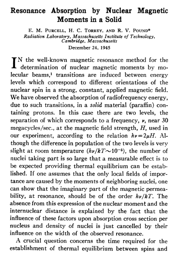
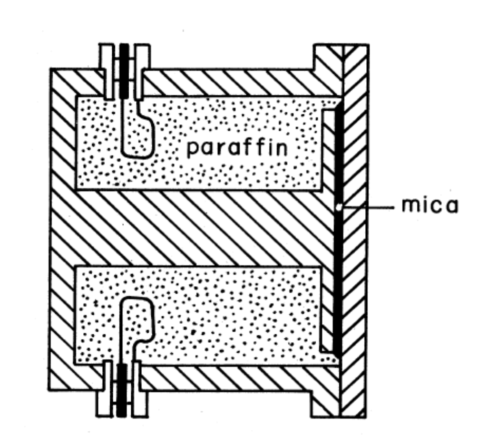

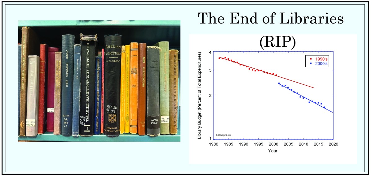

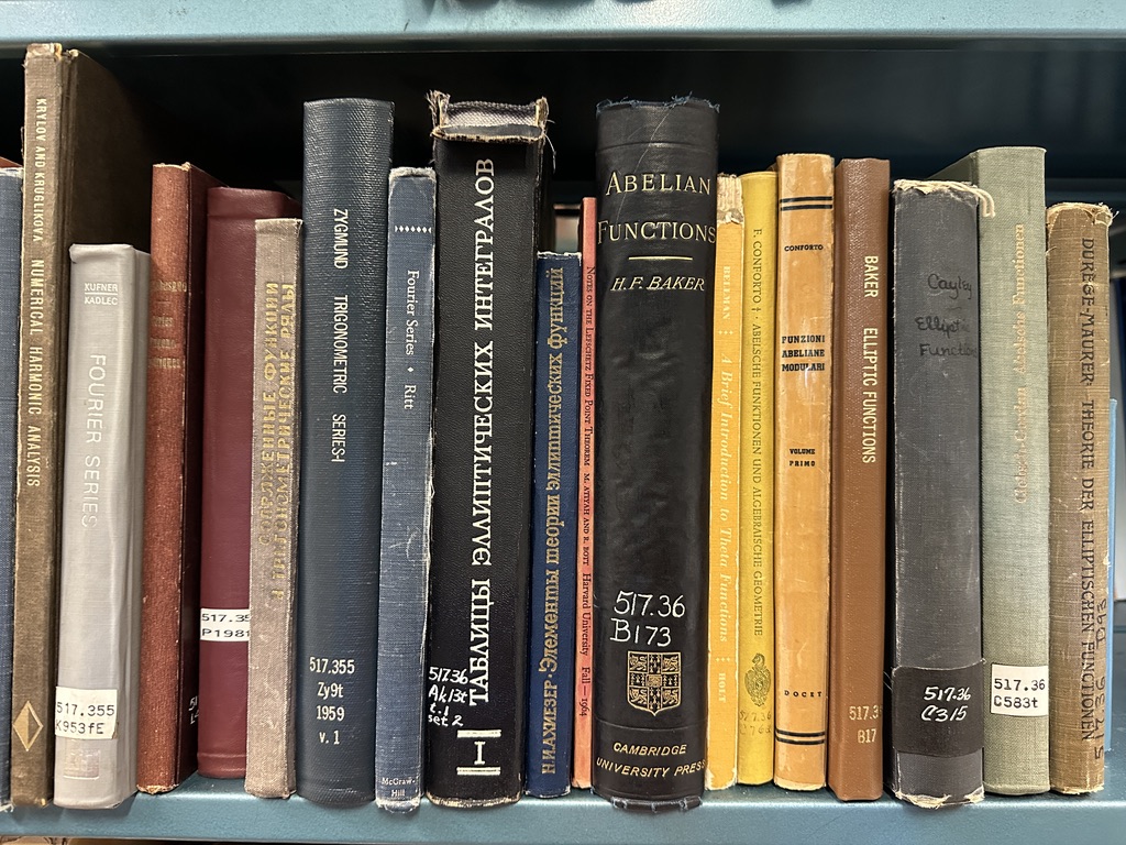
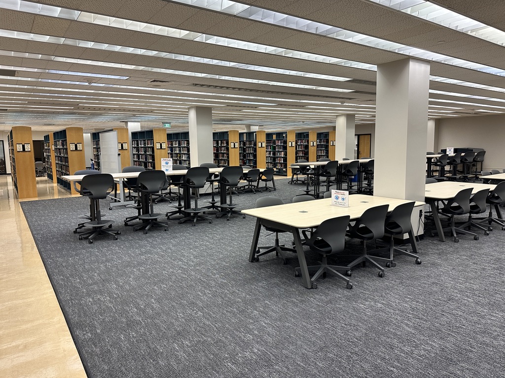

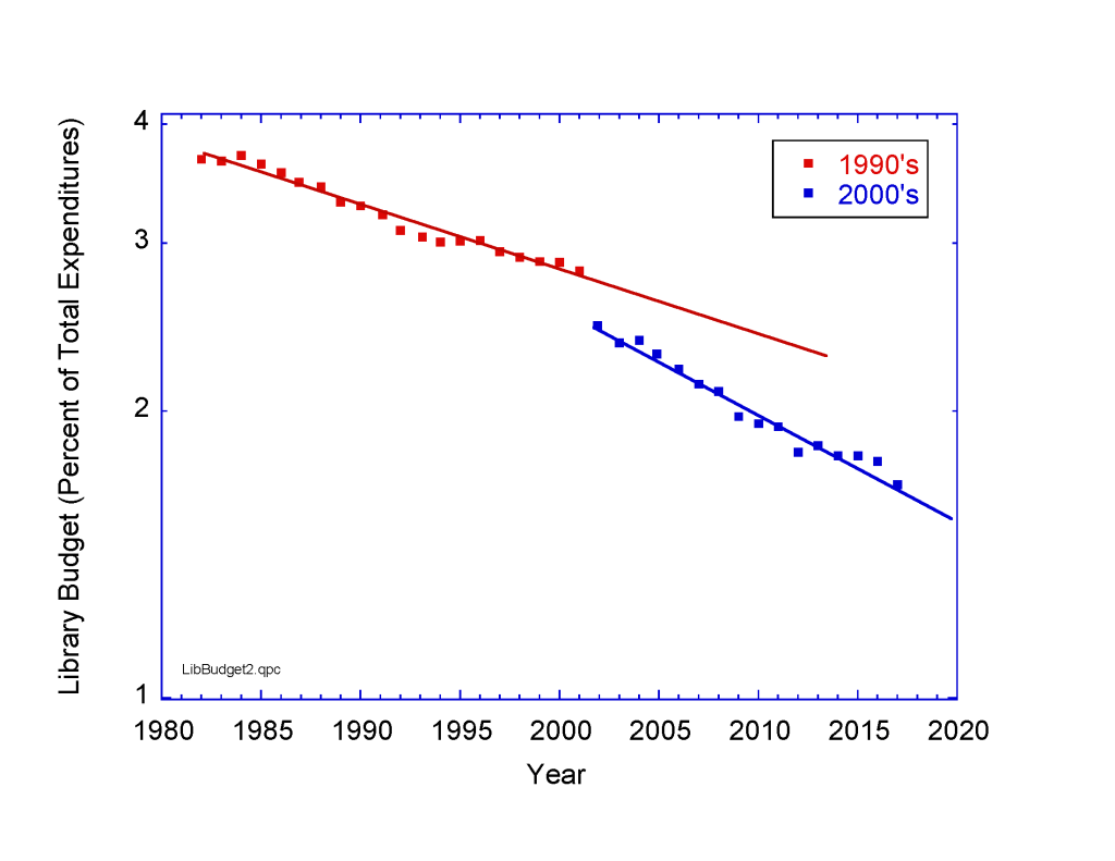
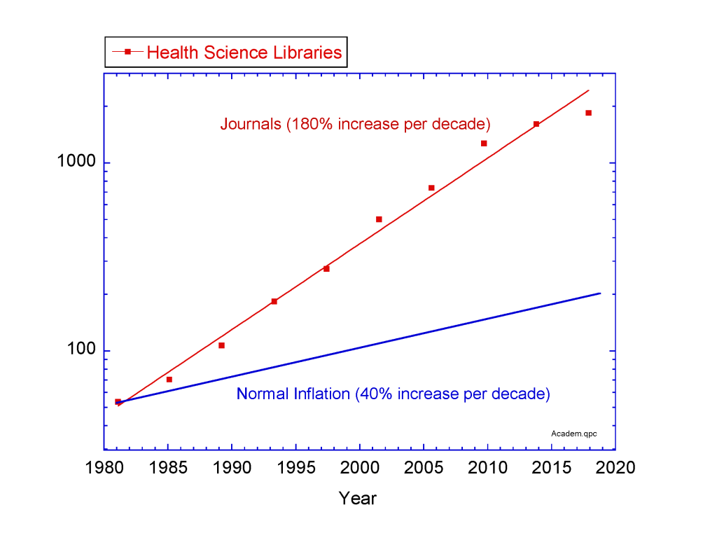

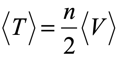
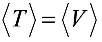
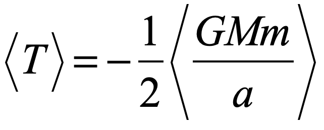
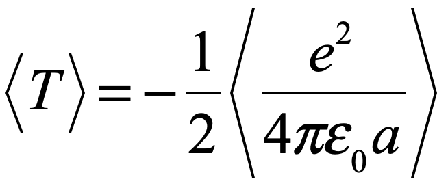
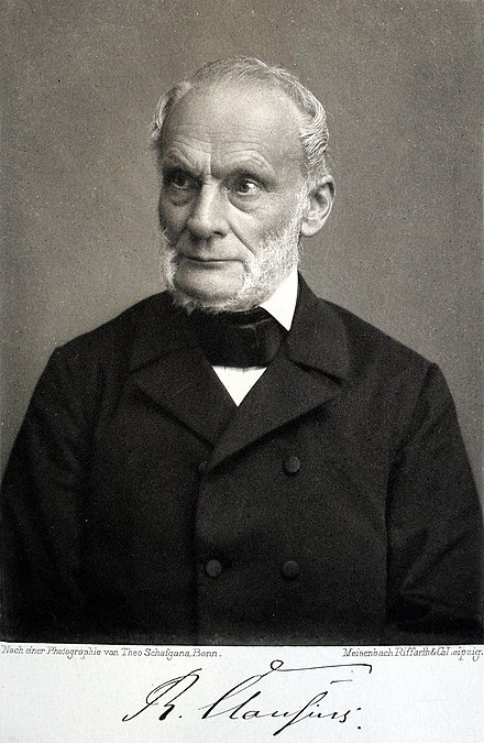
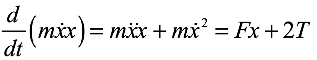
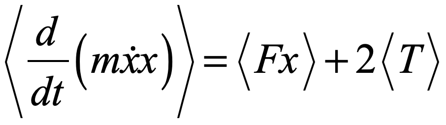
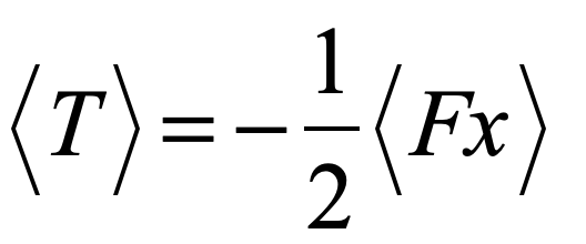
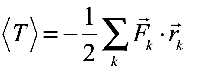
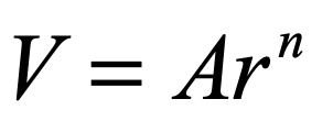
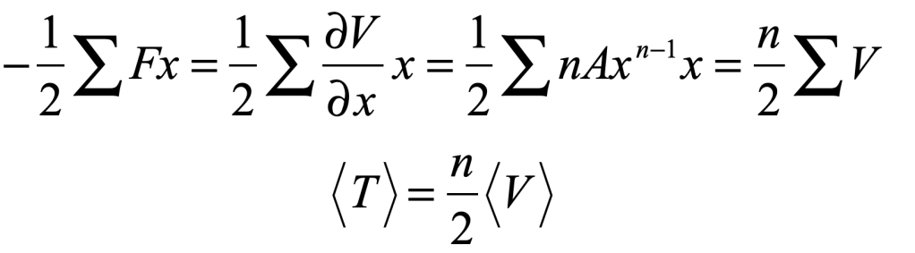

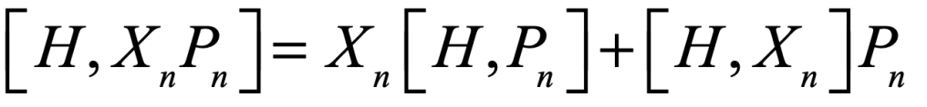
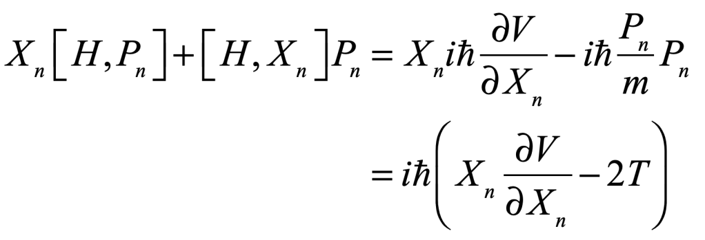
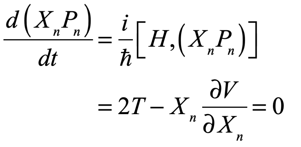

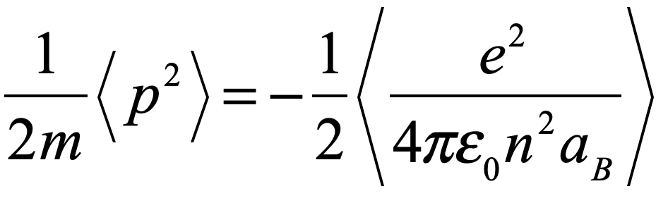
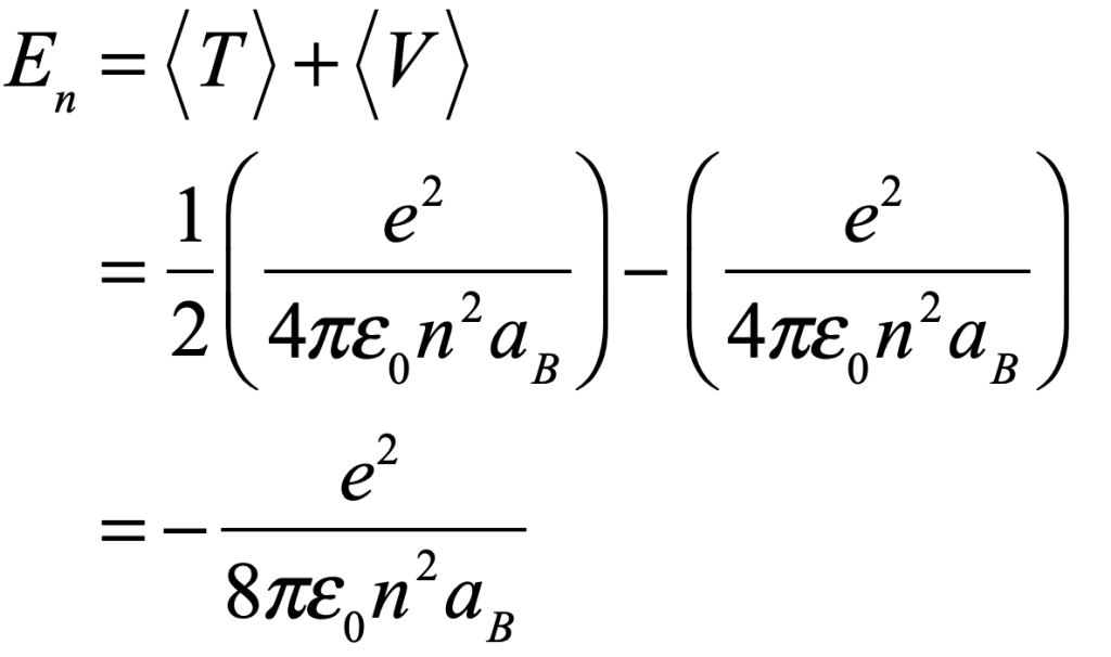


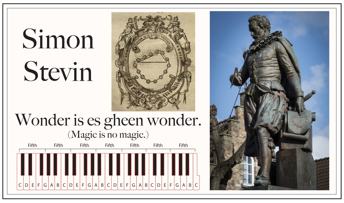
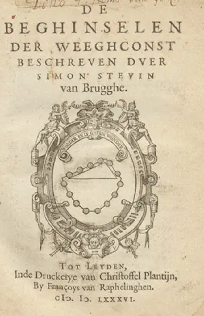

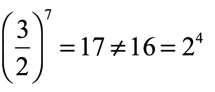
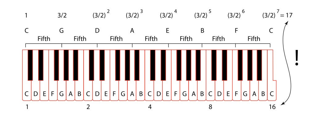
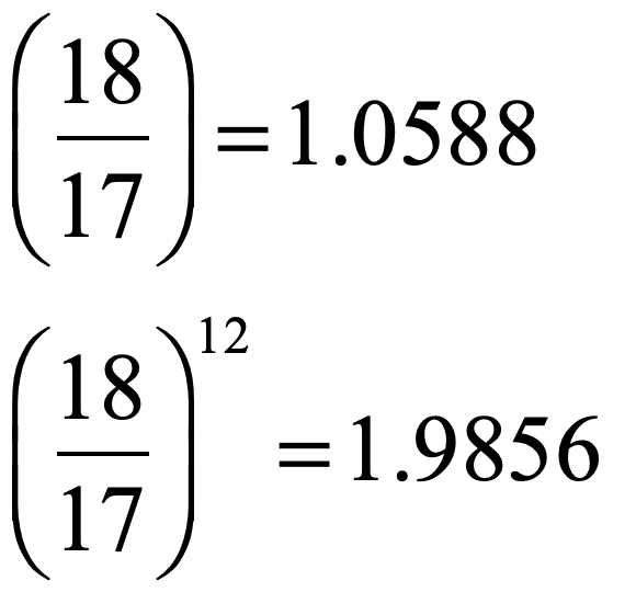
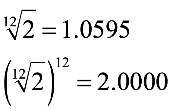

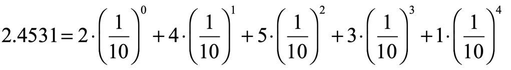
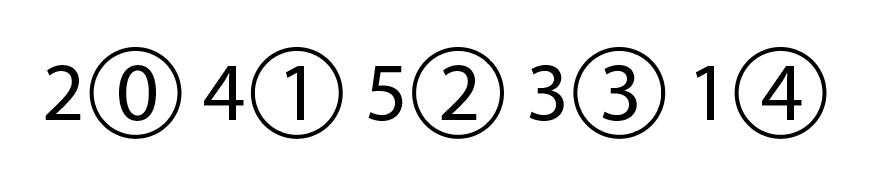


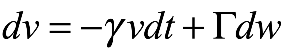
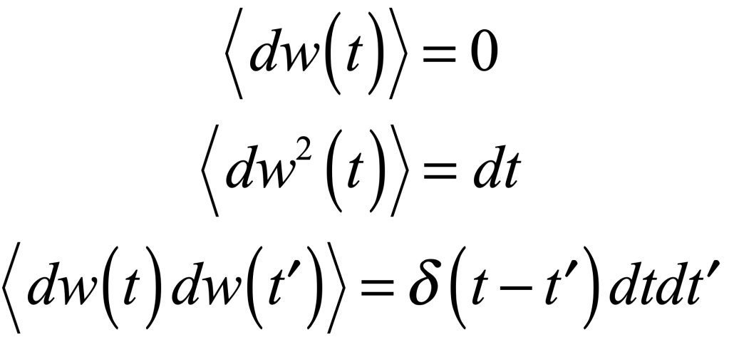


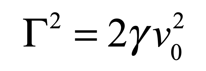
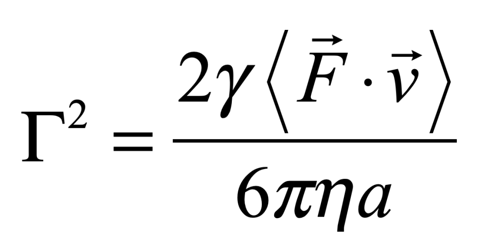
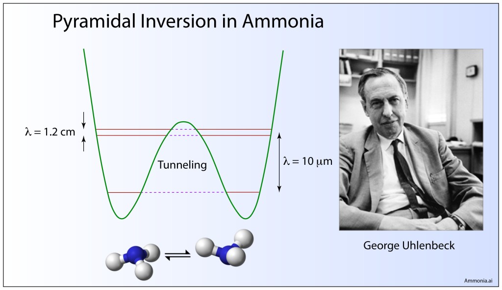


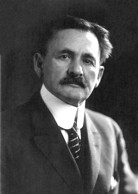

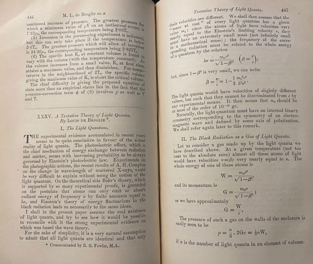


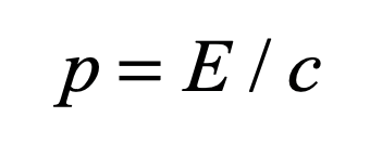

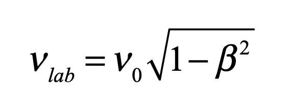


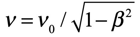
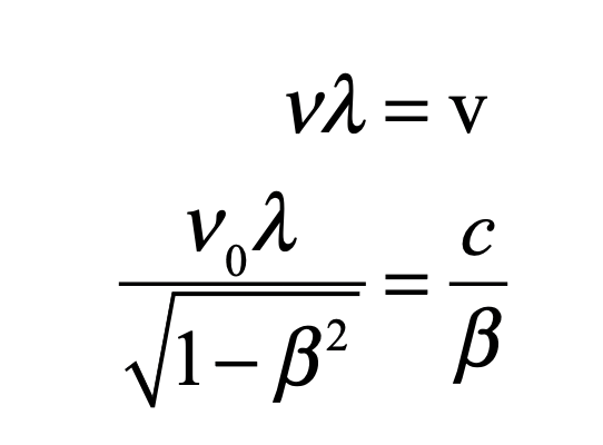

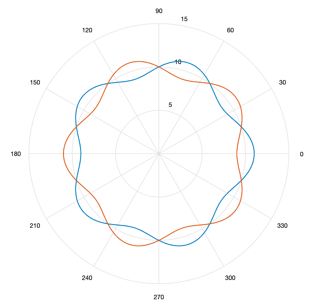
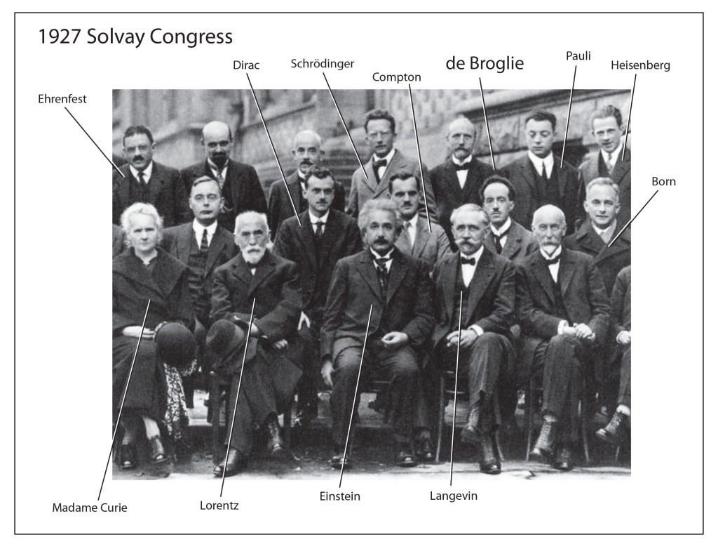


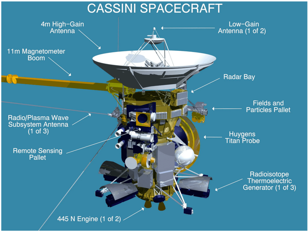
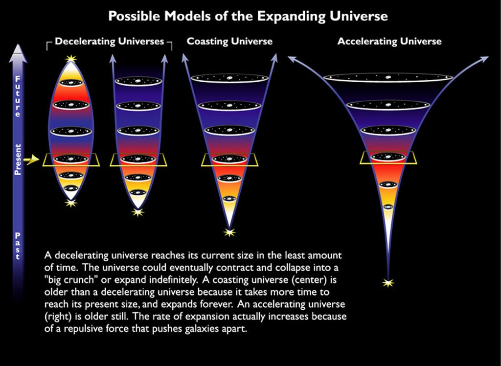
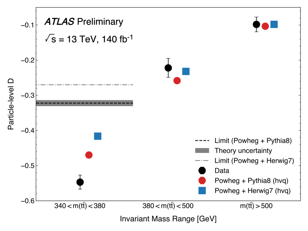
