Heisenberg’s uncertainty principle is a law of physics – it cannot be violated under any circumstances, no matter how much we may want it to yield or how hard we try to bend it. Heisenberg, as he developed his ideas after his lone epiphany like a monk on the isolated island of Helgoland off the north coast of Germany in 1925, became a bit of a zealot, like a religious convert, convinced that all we can say about reality is a measurement outcome. In his view, there was no independent existence of an electron other than what emerged from a measuring apparatus. Reality, to Heisenberg, was just a list of numbers in a spread sheet—matrix elements. He took this line of reasoning so far that he stated without exception that there could be no such thing as a trajectory in a quantum system. When the great battle commenced between Heisenberg’s matrix mechanics against Schrödinger’s wave mechanics, Heisenberg was relentless, denying any reality to Schrödinger’s wavefunction other than as a calculation tool. He was so strident that even Bohr, who was on Heisenberg’s side in the argument, advised Heisenberg to relent [1]. Eventually a compromise was struck, as Heisenberg’s uncertainty principle allowed Schrödinger’s wave functions to exist within limits—his uncertainty limits.
Disaster in the Poconos
Yet the idea of an actual trajectory of a quantum particle remained a type of heresy within the close quantum circles. Years later in 1948, when a young Richard Feynman took the stage at a conference in the Poconos, he almost sabotaged his career in front of Bohr and Dirac—two of the giants who had invented quantum mechanics—by having the audacity to talk about particle trajectories in spacetime diagrams.
Feynman was making his first presentation of a new approach to quantum mechanics that he had developed based on path integrals. The challenge was that his method relied on space-time graphs in which “unphysical” things were allowed to occur. In fact, unphysical things were required to occur, as part of the sum over many histories of his path integrals. For instance, a key element in the approach was allowing electrons to travel backwards in time as positrons, or a process in which the electron and positron annihilate into a single photon, and then the photon decays back into an electron-positron pair—a process that is not allowed by mass and energy conservation. But this is a possible history that must be added to Feynman’s sum.
It all looked like nonsense to the audience, and the talk quickly derailed. Dirac pestered him with questions that he tried to deflect, but Dirac persisted like a raven. A question was raised about the Pauli exclusion principle, about whether an orbital could have three electrons instead of the required two, and Feynman said that it could—all histories were possible and had to be summed over—an answer that dismayed the audience. Finally, as Feynman was drawing another of his space-time graphs showing electrons as lines, Bohr rose to his feet and asked derisively whether Feynman had forgotten Heisenberg’s uncertainty principle that made it impossible to even talk about an electron trajectory.
It was hopeless. The audience gave up and so did Feynman as the talk just fizzled out. It was a disaster. What had been meant to be Feynman’s crowning achievement and his entry to the highest levels of theoretical physics, had been a terrible embarrassment. He slunk home to Cornell where he sank into one of his depressions. At the close of the Pocono conference, Oppenheimer, the reigning king of physics, former head of the successful Manhattan Project and newly selected to head the prestigious Institute for Advanced Study at Princeton, had been thoroughly disappointed by Feynman.
But what Bohr and Dirac and Oppenheimer had failed to understand was that as long as the duration of unphysical processes was shorter than the energy differences involved, then it was literally obeying Heisenberg’s uncertainty principle. Furthermore, Feynman’s trajectories—what became his famous “Feynman Diagrams”—were meant to be merely cartoons—a shorthand way to keep track of lots of different contributions to a scattering process. The quantum processes certainly took place in space and time, conceptually like a trajectory, but only so far as time durations, and energy differences and locations and momentum changes were all within the bounds of the uncertainty principle. Feynman had invented a bold new tool for quantum field theory, able to supply deep results quickly. But no one at the Poconos could see it.
Fig. 1 The first Feynman diagram.
Coherent States
When Feynman had failed so miserably at the Pocono conference, he had taken the stage after Julian Schwinger, who had dazzled everyone with his perfectly scripted presentation of quantum field theory—the competing theory to Feynman’s. Schwinger emerged the clear winner of the contest. At that time, Roy Glauber (1925 – 2018) was a young physicist just taking his PhD from Schwinger at Harvard, and he later received a post-doc position at Princeton’s Institute for Advanced Study where he became part of a miniature revolution in quantum field theory that revolved around—not Schwinger’s difficult mathematics—but Feynman’s diagrammatic method. So Feynman won in the end. Glauber then went on to Caltech, where he filled in for Feynman’s lectures when Feynman was off in Brazil playing the bongos. Glauber eventually returned to Harvard where he was already thinking about the quantum aspects of photons in 1956 when news of the photon correlations in the Hanbury-Brown Twiss (HBT) experiment were published. Three years later, when the laser was invented, he began developing a theory of photon correlations in laser light that he suspected would be fundamentally different than in natural chaotic light.
Because of his background in quantum field theory, and especially quantum electrodynamics, it was fairly easy to couch the quantum optical properties of coherent light in terms of Dirac’s creation and annihilation operators of the electromagnetic field. Glauber developed a “coherent state” operator that was a minimum uncertainty state of the quantized electromagnetic field, related to the minimum-uncertainty wave functions derived initially by Schrödinger in the late 1920’s. The coherent state represents a laser operating well above the lasing threshold and behaved as “the most classical” wavepacket that can be constructed. Glauber was awarded the Nobel Prize in Physics in 2005 for his work on such “Glauber states” in quantum optics.
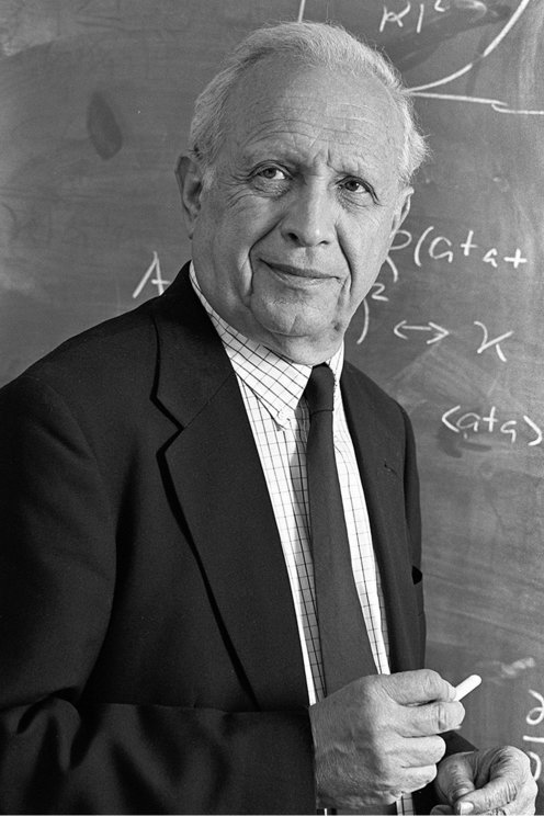
Fig. 2 Roy Glauber
Quantum Trajectories
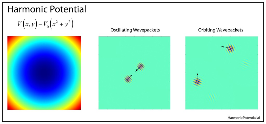
Glauber’s coherent states are built up from the natural modes of a harmonic oscillator. Therefore, it should come as no surprise that these coherent-state wavefunctions in a harmonic potential behave just like classical particles with well-defined trajectories. The quadratic potential matches the quadratic argument of the the Gaussian wavepacket, and the pulses propagate within the potential without broadening, as in Fig. 3, showing a snapshot of two wavepackets propagating in a two-dimensional harmonic potential. This is a somewhat radical situation, because most wavepackets in most potentials (or even in free space) broaden as they propagate. The quadratic potential is a special case that is generally not representative of how quantum systems behave.
Fig. 3 Harmonic potential in 2D and two examples of pairs of pulses propagating without broadening. The wavepackets in the center are oscillating in line, and the wavepackets on the right are orbiting the center of the potential in opposite directions. (Movies of the quantum trajectories can be viewed at Physics Unbound.)
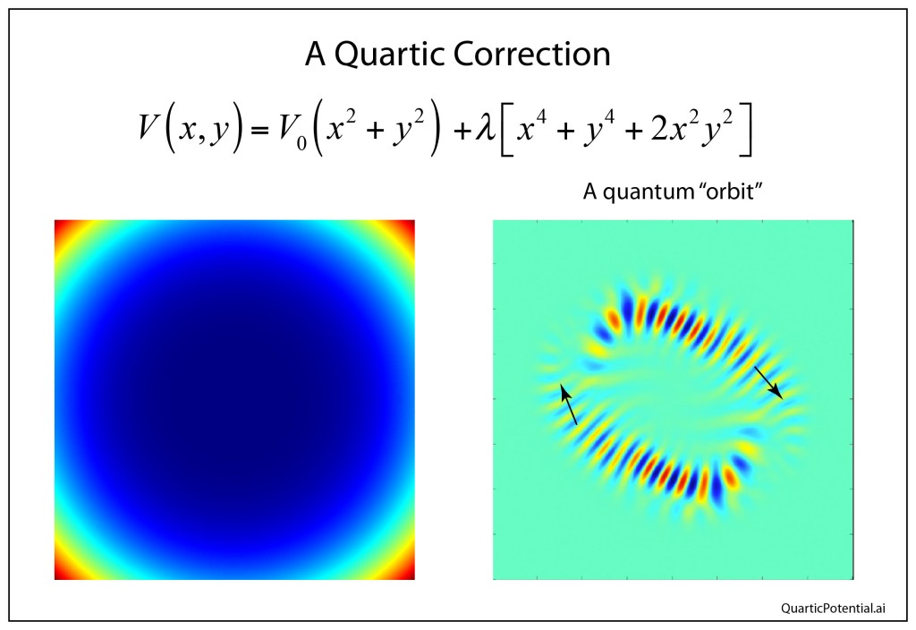
To illustrate this special status for the quadratic potential, the wavepackets can be launched in a potential with a quartic perturbation. The quartic potential is anharmonic—the frequency of oscillation depends on the amplitude of oscillation unlike for the harmonic oscillator, where amplitude and frequency are independent. The quartic potential is integrable, like the harmonic oscillator, and there is no avenue for chaos in the classical analog. Nonetheless, wavepackets broaden as they propagate in the quartic potential, eventually spread out into a ring in the configuration space, as in Fig. 4.
Fig. 4 Potential with a quartic corrections. The initial gaussian pulses spread into a “ring” orbiting the center of the potential.
A potential with integrability has as many conserved quantities to the motion as there are degrees of freedom. Because the quartic potential is integrable, the quantum wavefunction may spread, but it remains highly regular, as in the “ring” that eventually forms over time. However, integrable potentials are the exception rather than the rule. Most potentials lead to nonintegrable motion that opens the door to chaos.
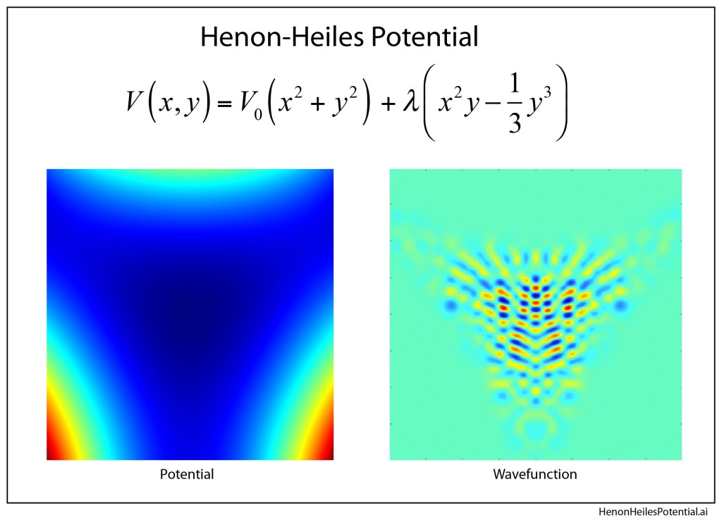
A classic (and classical) potential that exhibits chaos in a two-dimensional configuration space is the famous Henon-Heiles potential. This has a four-dimensional phase space which admits classical chaos. The potential has a three-fold symmetry which is one reason it is non-integral, since a particle must “decide” which way to go when it approaches a saddle point. In the quantum regime, wavepackets face the same decision, leading to a breakup of the wavepacket on top of a general broadening. This allows the wavefunction eventually to distribute across the entire configuration space, as in Fig. 5.
Fig. 5 The Henon-Heiles two-dimensional potential supports Hamiltonian chaos in the classical regime. In the quantum regime, the wavefunction spreads to eventually fill the accessible configuration space (for constant energy).
Youtube Video
Movies of quantum trajectories can be viewed at my Youtube Channel, Physics Unbound. The answer to the question “Is there a quantum trajectory?” can be seen visually as the movies run—they do exist in a very clear sense under special conditions, especially coherent states in a harmonic oscillator. And the concept of a quantum trajectory also carries over from a classical trajectory in cases when the classical motion is integrable, even in cases when the wavefunction spreads over time. However, for classical systems that display chaotic motion, wavefunctions that begin as coherent states break up into chaotic wavefunctions that fill the accessible configuration space for a given energy. The character of quantum evolution of coherent states—the most classical of quantum wavefunctions—in these cases reflects the underlying character of chaotic motion in the classical analogs. This process can be seen directly watching the movies as a wavepacket approaches a saddle point in the potential and is split. Successive splits of the multiple wavepackets as they interact with the saddle points is what eventually distributes the full wavefunction into its chaotic form.
Therefore, the idea of a “quantum trajectory”, so thoroughly dismissed by Heisenberg, remains a phenomenological guide that can help give insight into the behavior of quantum systems—both integrable and chaotic.
As a side note, the laws of quantum physics obey time-reversal symmetry just as the classical equations do. In the third movie of “A Quantum Ballet“, wavefunctions in a double-well potential are tracked in time as they start from coherent states that break up into chaotic wavefunctions. It is like watching entropy in action as an ordered state devolves into a disordered state. But at the half-way point of the movie, the imaginary part of the wavefunction has its sign flipped, and the dynamics continue. But now the wavefunctions move from disorder into an ordered state, seemingly going against the second law of thermodynamics. Flipping the sign of the imaginary part of the wavefunction at just one instant in time plays the role of a time-reversal operation, and there is no violation of the second law.
Alice’s disturbing adventures in Wonderland tumbled upon her like a string of accidents as she wandered a world of chaos. Rules were never what they seemed and shifted whenever they wanted. She even met a cat who grinned ear-to-ear and could disappear entirely, or almost entirely, leaving only its grin.
The vanishing Cheshire Cat reminds us of another famous cat—Arnold’s Cat—that introduced the ideas of stretching and folding of phase-space volumes in non-integrable Hamiltonian systems. But when Arnold’s Cat becomes a Quantum Cat, a central question remains: What happens to the chaotic behavior of the classical system … does it survive the transition to quantum mechanics? The answer is surprisingly like the grin of the Cheshire Cat—the cat vanishes, but the grin remains. In the quantum world of the Cheshire Cat, the grin of the classical cat remains even after the rest of the cat vanished.
The Cheshire Cat fades away, leaving only its grin, like a fine filament, as classical chaos fades into quantum, leaving behind a quantum scar.
The Quantum Mechanics of Classically Chaotic Systems
The simplest Hamiltonian systems are integrable—they have as many constants of the motion as degrees of freedom. This holds for quantum systems as well as for classical. There is also a strong correspondence between classical and quantum systems for the integrable cases—literally the Correspondence Principle—that states that quantum systems at high quantum number approach classical behavior. Even at low quantum numbers, classical resonances are mirrored by quantum eigenfrequencies that can show highly regular spectra.
But integrable systems are rare—surprisingly rare. Almost no real-world Hamiltonian system is integrable, because the real world warps the ideal. No spring can displace indefinitely, and no potential is perfectly quadratic. There are always real-world non-idealities that destroy one constant of the motion or another, opening the door to chaos.
When classical Hamiltonian systems become chaotic, they don’t do it suddenly. Almost all transitions to chaos in Hamiltonian systems are gradual. One of the best examples of this is the KAM theory that starts with invariant action integrals that generate invariant tori in phase space. As nonintegrable perturbations increase, the tori break up slowly into island chains of stability as chaos infiltrates the separatrixes—first as thin filaments of chaos surrounding the islands—then growing in width to take up more and more of phase space. Even when chaos is fully developed, small islands of stability can remain—the remnants of stable orbits of the unperturbed system.
When the classical becomes quantum, chaos softens. Quantum wave functions don’t like to be confined—they spread and they tunnel. The separatrix of classical chaos—that barrier between regions of phase space—cannot constrain the exponential tails of wave functions. And the origin of chaos itself—the homoclinic point of the separatrix—gets washed out. Then the regular orbits of the classical system reassert themselves, and they appear, like the vestige of the Cheshire Cat, as a grin.
The Quantum Circus
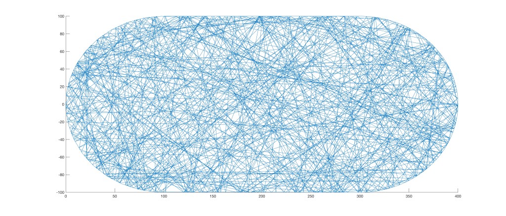
The empty stadium is a surprisingly rich dynamical system that has unexpected structure in both the classical and the quantum domain. Its importance in classical dynamics comes from the fact that its periodic orbits are unstable and its non-periodic orbits are ergodic (filling all available space if given long enough). The stadium itself is empty so that particles (classical or quantum) are free to propagate between reflections from the perfectly-reflecting walls of the stadium. The ergodicity comes from the fact that the stadium—like a classic Roman chariot-race stadium, also known as a circus—is not a circle, but has a straight stretch between two half circles. This simple modification takes the stable orbits of the circle into the unstable orbits of the stadium.
A single classical orbit in a stadium is shown in Fig 1. This is an ergodic orbit that is non-periodic and eventually would fill the entire stadium space. There are other orbits that are nearly periodic, such as one that bounces back and forth vertically between the linear portions, but even this orbit will eventually wander into the circular part of the stadium and then become ergodic. The big quantum-classical question is what happens to these classical orbits when the stadium is shrunk to the nanoscale?
Fig. 1 A classical trajectory in a stadium. It will eventually visit every point, a property known as ergodicity.
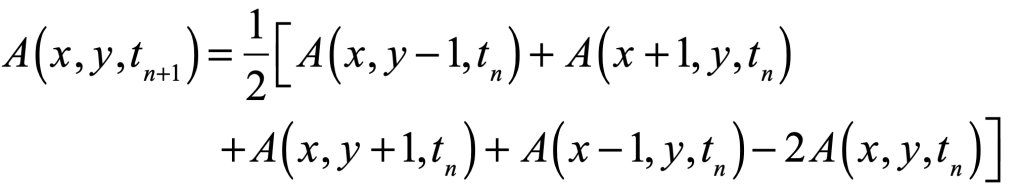
Simulating an evolving quantum wavefunction in free space is surprisingly simple. Given a beginning quantum wavefunction A(x,y,t0), the discrete update equation is
Perfect reflection from the boundaries of the stadium are incorporated through imposing a boundary condition that sends the wavefunction to zero. Simple!
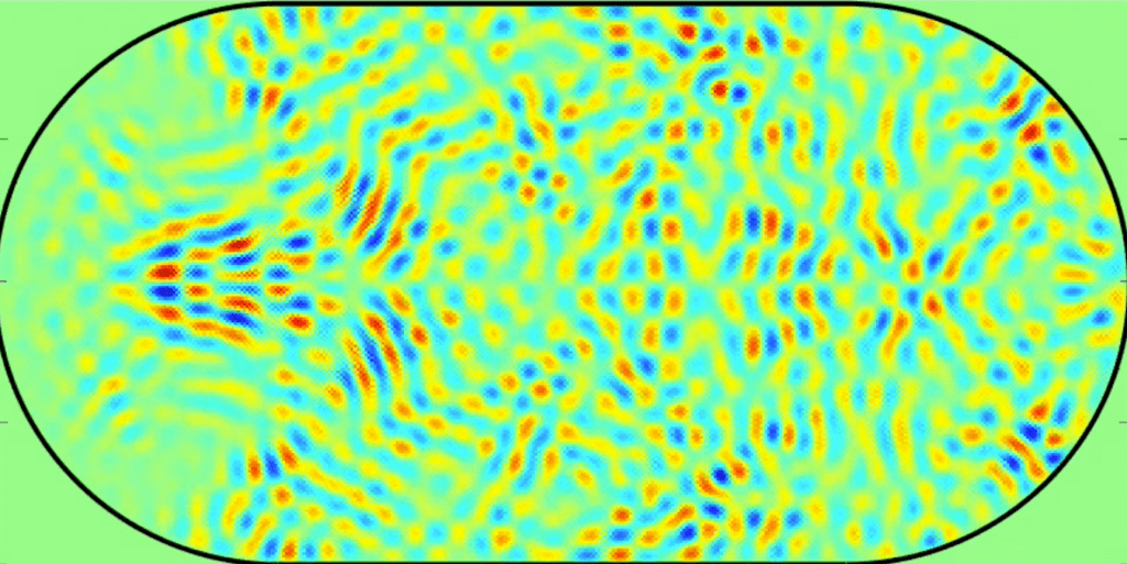
A snap-shot of a wavefunction evolving in the stadium is shown in Fig. 2. To see a movie of the time evolution, see my YouTube episode.
Fig. 2 Snapshot of a quantum wavefunction in the stadium. (From YouTube)
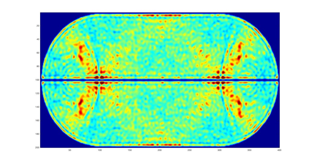
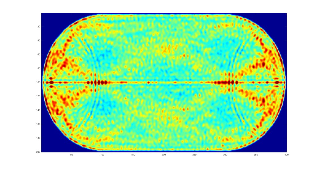
The time average of the wavefunction after a long time has passed is shown in Fig. 3. Other than the horizontal nodal line down the center of the stadium, there is little discernible structure or symmetry. This is also true for the mean squared wavefunction shown in Fig. 4, although there is some structure that may be emerging in the semi-circular regions.
Fig. 3 Time-average wavefunction after a long time.
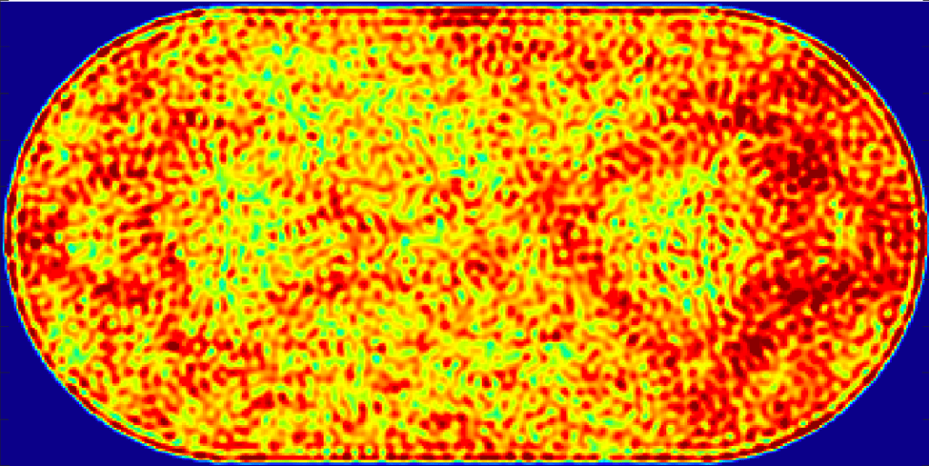
Fig. 4 Time-average of the squared wavefunction after a long time.
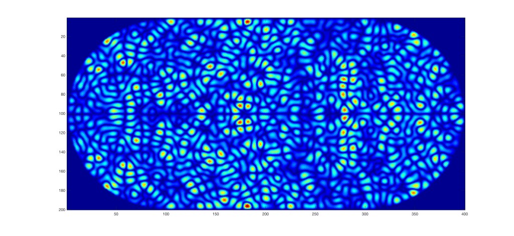
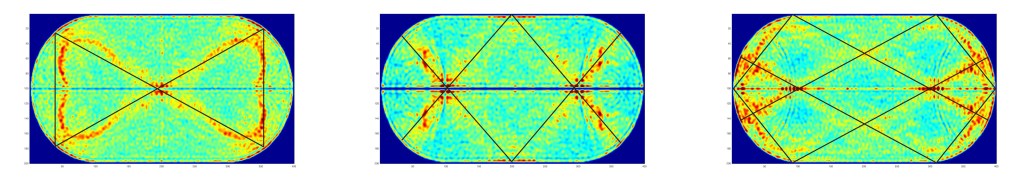
On the other hand, for special initial conditions that have a lot of symmetry, something remarkable happens. Fig. 5 shows several mean-squared results for special initial conditions. There is definite structure in these cases that were given the somewhat ugly name “quantum scars” in the 1980’s by Eric Heller who was one of the first to study this phenomenon [1].
Quantum ScarsQuantum ScarsQuantum Scars
Fig. 5 Quantum scars reflect periodic (but unstable) orbits of the classical system. Quantum effects tend to quench chaos and favor regular motion.
One can superpose highly-symmetric classical trajectories onto the figures, as shown in the bottom row. All of these classical orbits go through a high-symmetry point, such as the center of the stadium (on the left image) and through the focal point of the circular mirrors (in the other two images). The astonishing conclusion of this exercise is that the highly-symmetric periodic classical orbits remain behind as quantum scars—like the Cheshire Cat’s grin—when the system is in the quantum realm. The classical orbits that produce quantum scars have the important property of being periodic but unstable. A slight perturbation from the symmetric trajectory causes it to eventually become ergodic (chaotic). These scars are regions with enhanced probability density, what might be termed “quantum trajectories”, but do not show strong interference patterns.
It is important to make the distinction that it is also possible to construct special wavefunctions that are strictly periodic, such as a wave bouncing perfectly vertically between the straight portions. This leads to large-scale interference patterns that are not the same as the quantum scars.
Quantum Chaos versus Laser Speckle
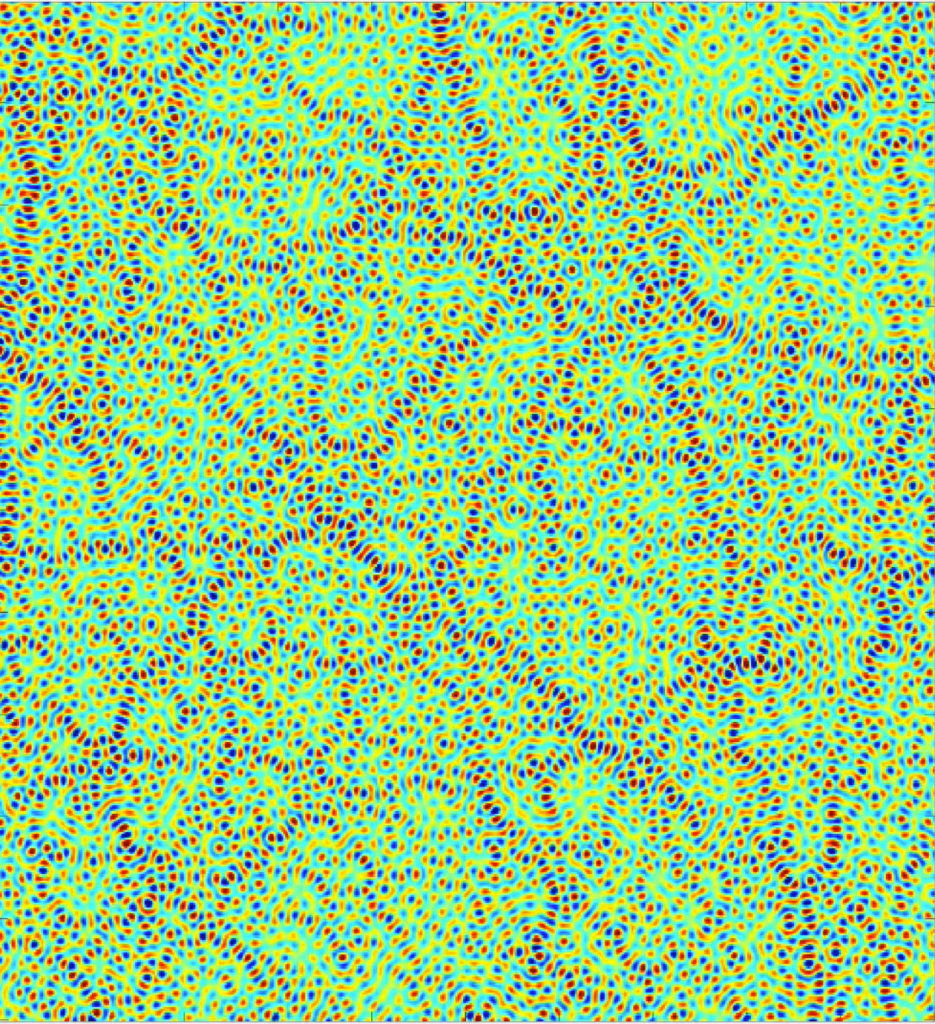
In addition to the bouncing-wave cases that do not strictly produce quantum scars, there is another “neutral” phenomenon that produces interference patterns that look a lot like scars, but are simply the random addition of lots of plane waves with the same wavelength [2]. A snapshot in time of one of these superpositions is shown in Fig. 6. To see how the waves add together, see the YouTube channel episode.
Fig. 6 The sum of 100 randomly oriented plane waves of constant wavelength. (A snapshot from YouTube.)
By David D. Nolte, Aug. 14, 2022
YouTube Video
Read more about the history of chaos theory in Galileo Unbound from Oxford Press:
In one interpretation of quantum physics, when you snap your fingers, the trajectory you are riding through reality fragments into a cascade of alternative universes—one for each possible quantum outcome among all the different quantum states composing the molecules of your fingers.
This is the Many-Worlds Interpretation (MWI) of quantum physics first proposed rigorously by Hugh Everett in his doctoral thesis in 1957 under the supervision of John Wheeler at Princeton University. Everett had been drawn to this interpretation when he found inconsistencies between quantum physics and gravitation—topics which were supposed to have been his actual thesis topic. But his side-trip into quantum philosophy turned out to be a one-way trip. The reception of his theory was so hostile, no less than from Copenhagen and Bohr himself, that Everett left physics and spent a career at the Pentagon.
Resurrecting MWI in the Name of Quantum Information
Fast forward by 20 years, after Wheeler had left Princeton for the University of Texas at Austin, and once again a young physicist was struggling to reconcile quantum physics with gravity. Once again the many worlds interpretation of quantum physics seemed the only sane way out of the dilemma, and once again a side-trip became a life-long obsession.
David Deutsch, visiting Wheeler in the early 1980’s, became convinced that the many worlds interpretation of quantum physics held the key to paradoxes in the theory of quantum information (For the full story of Wheeler, Everett and Deutsch, see Ref [1]). He was so convinced, that he began a quest to find a physical system that operated on more information than could be present in one universe at a time. If such a physical system existed, it would be because streams of information from more than one universe were coming together and combining in a way that allowed one of the universes to “borrow” the information from the other.
It took only a year or two before Deutsch found what he was looking for—a simple quantum algorithm that yielded twice as much information as would be possible if there were no parallel universes. This is the now-famous Deutsch algorithm—the first quantum algorithm [2]. At the heart of the Deutsch algorithm is a simple quantum interference. The algorithm did nothing useful—but it convinced Deutsch that two universes were interfering coherently in the measurement process, giving that extra bit of information that should not have been there otherwise. A few years later, the Deutsch-Josza algorithm [2] expanded the argument to interfere an exponentially larger amount of information streams from an exponentially larger number of universes to create a result that was exponentially larger than any classical computer could produce. This marked the beginning of the quest for the quantum computer that is running red-hot today.
Deutsch’s “proof” of the many-worlds interpretation of quantum mechanics is not a mathematical proof but is rather a philosophical proof. It holds no sway over how physicists do the math to make their predictions. The Copenhagen interpretation, with its “spooky” instantaneous wavefunction collapse, works just fine predicting the outcome of quantum algorithms and the exponential quantum advantage of quantum computing. Therefore, the story of David Deutsch and the MWI may seem like a chimera—except for one fact—it inspired him to generate the first quantum algorithm that launched what may be the next revolution in the information revolution of modern society. Inspiration is important in science, because it lets scientists create things that had been impossible before.
But if quantum interference is the heart of quantum computing, then there is one physical system that has the ultimate simplicity that may yet inspire future generations of physicists to invent future impossible things—the quantum beam splitter. Nothing in the study of quantum interference can be simpler than a sliver of dielectric material sending single photons one way or another. Yet the outcome of this simple system challenges the mind and reminds us of why Everett and Deutsch embraced the MWI in the first place.
The Classical Beam Splitter
The so-called “beam splitter” is actually a misnomer. Its name implies that it takes a light beam and splits it into two, as if there is only one input. But every “beam splitter” has two inputs, which is clear by looking at the classical 50/50 beam splitter. The actual action of the optical element is the combination of beams into superpositions in each of the outputs. It is only when one of the input fields is zero, a special case, that the optical element acts as a beam splitter. In general, it is a beam combiner.
Given two input fields, the output fields are superpositions of the inputs
The square-root of two factor ensures that energy is conserved, because optical fluence is the square of the fields. This relation is expressed more succinctly as a matrix input-output relation
The phase factors in these equations ensure that the matrix is unitary
reflecting energy conservation.
The Quantum Beam Splitter
A quantum beam splitter is just a classical beam splitter operating at the level of individual photons. Rather than describing single photons entering or leaving the beam splitter, it is more practical to describe the properties of the fields through single-photon quantum operators
where the unitary matrix is the same as the classical case, but with fields replaced by the famous “a” operators. The photon operators operate on single photon modes. For instance, the two one-photon input cases are
where the creation operators operate on the vacuum state in each of the input modes.
The fundamental combinational properties of the beam splitter are even more evident in the quantum case, because there is no such thing as a single input to a quantum beam splitter. Even if no photons are directed into one of the input ports, that port still receives a “vacuum” input, and this vacuum input contributes to the fluctuations observed in the outputs.
The input-output relations for the quantum beam splitter are
The beam splitter operating on a one-photon input converts the input-mode creation operator into a superposition of out-mode creation operators that generates
The resulting output is entangled: either the single photon exits one port, or it exits the other. In the many worlds interpretation, the photon exits from one port in one universe, and it exits from the other port in a different universe. On the other hand, in the Copenhagen interpretation, the two output ports of the beam splitter are perfectly anti-correlated.
Fig. 1 Quantum Operations of a Beam Splitter. A beam splitter creates a quantum superposition of the input modes. The a-symbols are quantum number operators that create and annihilate photons. A single-photon input produces an entangled output that is a quantum superposition of the photon coming out of one output or the other.
The Hong-Ou-Mandel (HOM) Interferometer
When more than one photon is incident on a beam splitter, the fascinating effects of quantum interference come into play, creating unexpected outputs for simple inputs. For instance, the simplest example is a two photon input where a single photon is present in each input port of the beam splitter. The input state is represented with single creation operators operating on each vacuum state of each input port
creating a single photon in each of the input ports. The beam splitter operates on this input state by converting the input-mode creation operators into out-put mode creation operators to give
The important step in this process is the middle line of the equations: There is perfect destructive interference between the two single-photon operations. Therefore, both photons always exit the beam splitter from the same port—never split. Furthermore, the output is an entangled two-photon state, once more splitting universes.
Fig. 2 The HOM interferometer. A two-photon input on a beam splitter generates an entangled superposition of the two photons exiting the beam splitter always together.
The two-photon interference experiment was performed in 1987 by Chung Ki Hong and Jeff Ou, students of Leonard Mandel at the Optics Institute at the University of Rochester [4], and this two-photon operation of the beam splitter is now called the HOM interferometer. The HOM interferometer has become a center-piece for optical and photonic implementations of quantum information processing and quantum computers.
N-Photons on a Beam Splitter
Of course, any number of photons can be input into a beam splitter. For example, take the N-photon input state
The beam splitter acting on this state produces
The quantity on the right hand side can be re-expressed using the binomial theorem
where the permutations are defined by the binomial coefficient
The output state is given by
which is a “super” entangled state composed of N multi-photon states, involving N different universes.
Coherent States on a Quantum Beam Splitter
Surprisingly, there is a multi-photon input state that generates a non-entangled output—as if the input states were simply classical fields. These are the so-called coherent states, introduced by Glauber and Sudarshan [5, 6]. Coherent states can be described as superpositions of multi-photon states, but when a beam splitter operates on these superpositions, the outputs are simply 50/50 mixtures of the states. For instance, if the input scoherent tates are denoted by α and β, then the output states after the beam splitter are
This output is factorized and hence is NOT entangled. This is one of the many reasons why coherent states in quantum optics are considered the “most classical” of quantum states. In this case, a quantum beam splitter operates on the inputs just as if they were classical fields.
By David D. Nolte, May 8, 2022
Read more in “Interference” (New from Oxford University Press, 2023)
A popular account of the trials and toils of the scientists and engineers who tamed light and used it to probe the universe.
[2] D. Deutsch, “Quantum-theory, the church-turing principle and the universal quantum computer,” Proceedings of the Royal Society of London Series a-Mathematical Physical and Engineering Sciences, vol. 400, no. 1818, pp. 97-117, (1985)
[3] D. Deutsch and R. Jozsa, “Rapid solution of problems by quantum computation,” Proceedings of the Royal Society of London Series a-Mathematical Physical and Engineering Sciences, vol. 439, no. 1907, pp. 553-558, Dec (1992)
[4] C. K. Hong, Z. Y. Ou, and L. Mandel, “Measurement of subpicosecond time intervals between 2 photons by interference,” Physical Review Letters, vol. 59, no. 18, pp. 2044-2046, Nov (1987)
[5] Glauber, R. J. (1963). “Photon Correlations.” Physical Review Letters 10(3): 84.
[6] Sudarshan, E. C. G. (1963). “Equivalence of semiclassical and quantum mechanical descriptions of statistical light beams.” Physical Review Letters 10(7): 277-&.; Mehta, C. L. and E. C. Sudarshan (1965). “Relation between quantum and semiclassical description of optical coherence.” Physical Review 138(1B): B274.
Now is exactly the wrong moment to be reviewing the state of photonic quantum computing — the field is moving so rapidly, at just this moment, that everything I say here now will probably be out of date in just a few years. On the other hand, now is exactly the right time to be doing this review, because so much has happened in just the past few years, that it is important to take a moment and look at where this field is today and where it will be going.
At the 20-year anniversary of the publication of my book Mind at Light Speed (Free Press, 2001), this blog is the third in a series reviewing progress in three generations of Machines of Light over the past 20 years (see my previous blogs on the future of the photonic internet and on all-optical computers). This third and final update reviews progress on the third generation of the Machines of Light: the Quantum Optical Generation. Of the three generations, this is the one that is changing the fastest.
Quantum computing is almost here … and it will be at room temperature, using light, in photonic integrated circuits!
Quantum Computing with Linear Optics
Twenty years ago in 2001, Emanuel Knill and Raymond LaFlamme at Los Alamos National Lab, with Gerald Mulburn at the University of Queensland, Australia, published a revolutionary theoretical paper (known as KLM) in Nature on quantum computing with linear optics: “A scheme for efficient quantum computation with linear optics” [1]. Up until that time, it was believed that a quantum computer — if it was going to have the property of a universal Turing machine — needed to have at least some nonlinear interactions among qubits in a quantum gate. For instance, an example of a two-qubit gate is a controlled-NOT, or CNOT, gate shown in Fig. 1 with the Truth Table and the equivalent unitary matrix. It clear that one qubit is controlling the other, telling it what to do.
The quantum CNOT gate gets interesting when the control line has a quantum superposition, then the two outputs become entangled.
Entanglement is a strange process that is unique to quantum systems and has no classical analog. It also has no simple intuitive explanation. By any normal logic, if the control line passes through the gate unaltered, then absolutely nothing interesting should be happening on the Control-Out line. But that’s not the case. The control line going in was a separate state. If some measurement were made on it, either a 1 or 0 would be seen with equal probability. But coming out of the CNOT, the signal has somehow become perfectly correlated with whatever value is on the Signal-Out line. If the Signal-Out is measured, the measurement process collapses the state of the Control-Out to a value equal to the measured signal. The outcome of the control line becomes 100% certain even though nothing was ever done to it! This entanglement generation is one reason the CNOT is often the gate of choice when constructing quantum circuits to perform interesting quantum algorithms.
However, optical implementation of a CNOT is a problem, because light beams and photons really do not like to interact with each other. This is the problem with all-optical classical computers too (see my previous blog). There are ways of getting light to interact with light, for instance inside nonlinear optical materials. And in the case of quantum optics, a single atom in an optical cavity can interact with single photons in ways that can act like a CNOT or related gates. But the efficiencies are very low and the costs to implement it are very high, making it difficult or impossible to scale such systems up into whole networks needed to make a universal quantum computer.
Therefore, when KLM published their idea for quantum computing with linear optics, it caused a shift in the way people were thinking about optical quantum computing. A universal optical quantum computer could be built using just light sources, beam splitters and photon detectors.
The way that KLM gets around the need for a direct nonlinear interaction between two photons is to use postselection. They run a set of photons — signal photons and ancilla (test) photons — through their linear optical system and they detect (i.e., theoretically…the paper is purely a theoretical proposal) the ancilla photons. If these photons are not detected where they are wanted, then that iteration of the computation is thrown out, and it is tried again and again, until the photons end up where they need to be. When the ancilla outcomes are finally what they need to be, this run is selected because the signal state are known to have undergone a known transformation. The signal photons are still unmeasured at this point and are therefore in quantum superpositions that are useful for quantum computation. Postselection uses entanglement and measurement collapse to put the signal photons into desired quantum states. Postselection provides an effective nonlinearity that is induced by the wavefunction collapse of the entangled state. Of course, the down side of this approach is that many iterations are thrown out — the computation becomes non-deterministic.
KLM could get around most of the non-determinism by using more and more ancilla photons, but this has the cost of blowing up the size and cost of the implementation, so their scheme was not imminently practical. But the important point was that it introduced the idea of linear quantum computing. (For this, Milburn and his collaborators have my vote for a future Nobel Prize.) Once that idea was out, others refined it, and improved upon it, and found clever ways to make it more efficient and more scalable. Many of these ideas relied on a technology that was co-evolving with quantum computing — photonic integrated circuits (PICs).
Quantum Photonic Integrated Circuits (QPICs)
Never underestimate the power of silicon. The amount of time and energy and resources that have now been invested in silicon device fabrication is so astronomical that almost nothing in this world can displace it as the dominant technology of the present day and the future. Therefore, when a photon can do something better than an electron, you can guess that eventually that photon will be encased in a silicon chip–on a photonic integrated circuit (PIC).
The dream of integrated optics (the optical analog of integrated electronics) has been around for decades, where waveguides take the place of conducting wires, and interferometers take the place of transistors — all miniaturized and fabricated in the thousands on silicon wafers. The advantages of PICs are obvious, but it has taken a long time to develop. When I was a post-doc at Bell Labs in the late 1980’s, everyone was talking about PICs, but they had terrible fabrication challenges and terrible attenuation losses. Fortunately, these are just technical problems, not limited by any fundamental laws of physics, so time (and an army of researchers) has chipped away at them.
One of the driving forces behind the maturation of PIC technology is photonic fiber optic communications (as discussed in a previous blog). Photons are clear winners when it comes to long-distance communications. In that sense, photonic information technology is a close cousin to silicon — photons are no less likely to be replaced by a future technology than silicon is. Therefore, it made sense to bring the photons onto the silicon chips, tapping into the full array of silicon fab resources so that there could be seamless integration between fiber optics doing the communications and the photonic chips directing the information. Admittedly, photonic chips are not yet all-optical. They still use electronics to control the optical devices on the chip, but this niche for photonics has provided a driving force for advancements in PIC fabrication.
Fig. 2 Schematic of a silicon photonic integrated circuit (PIC). The waveguides can be silica or nitride deposited on the silicon chip. From the Comsol WebSite.
One side-effect of improved PIC fabrication is low light losses. In telecommunications, this loss is not so critical because the systems use OEO regeneration. But less loss is always good, and the PICs can now safeguard almost every photon that comes on chip — exactly what is needed for a quantum PIC. In a quantum photonic circuit, every photon is valuable and informative and needs to be protected. The new PIC fabrication can do this. In addition, light switches for telecom applications are built from integrated interferometers on the chip. It turns out that interferometers at the single-photon level are unitary quantum gates that can be used to build universal photonic quantum computers. So the same technology and control that was used for telecom is just what is needed for photonic quantum computers. In addition, integrated optical cavities on the PICs, which look just like wavelength filters when used for classical optics, are perfect for producing quantum states of light known as squeezed light that turn out to be valuable for certain specialty types of quantum computing.
Therefore, as the concepts of linear optical quantum computing advanced through that last 20 years, the hardware to implement those concepts also advanced, driven by a highly lucrative market segment that provided the resources to tap into the vast miniaturization capabilities of silicon chip fabrication. Very fortuitous!
Room-Temperature Quantum Computers
There are many radically different ways to make a quantum computer. Some are built of superconducting circuits, others are made from semiconductors, or arrays of trapped ions, or nuclear spins on nuclei on atoms in molecules, and of course with photons. Up until about 5 years ago, optical quantum computers seemed like long shots. Perhaps the most advanced technology was the superconducting approach. Superconducting quantum interference devices (SQUIDS) have exquisite sensitivity that makes them robust quantum information devices. But the drawback is the cold temperatures that are needed for them to work. Many of the other approaches likewise need cold temperature–sometimes astronomically cold temperatures that are only a few thousandths of a degree above absolute zero Kelvin.
Cold temperatures and quantum computing seemed a foregone conclusion — you weren’t ever going to separate them — and for good reason. The single greatest threat to quantum information is decoherence — the draining away of the kind of quantum coherence that allows interferences and quantum algorithms to work. In this way, entanglement is a two-edged sword. On the one hand, entanglement provides one of the essential resources for the exponential speed-up of quantum algorithms. But on the other hand, if a qubit “sees” any environmental disturbance, then it becomes entangled with that environment. The entangling of quantum information with the environment causes the coherence to drain away — hence decoherence. Hot environments disturb quantum systems much more than cold environments, so there is a premium for cooling the environment of quantum computers to as low a temperature as they can. Even so, decoherence times can be microseconds to milliseconds under even the best conditions — quantum information dissipates almost as fast as you can make it.
Enter the photon! The bottom line is that photons don’t interact. They are blind to their environment. This is what makes them perfect information carriers down fiber optics. It is also what makes them such good qubits for carrying quantum information. You can prepare a photon in a quantum superposition just by sending it through a lossless polarizing crystal, and then the superposition will last for as long as you can let the photon travel (at the speed of light). Sometimes this means putting the photon into a coil of fiber many kilometers long to store it, but that is OK — a kilometer of coiled fiber in the lab is no bigger than a few tens of centimeters. So the same properties that make photons excellent at carrying information also gives them very small decoherence. And after the KLM schemes began to be developed, the non-interacting properties of photons were no longer a handicap.
In the past 5 years there has been an explosion, as well as an implosion, of quantum photonic computing advances. The implosion is the level of integration which puts more and more optical elements into smaller and smaller footprints on silicon PICs. The explosion is the number of first-of-a-kind demonstrations: the first universal optical quantum computer [2], the first programmable photonic quantum computer [3], and the first (true) quantum computational advantage [4].
All of these “firsts” operate at room temperature. (There is a slight caveat: The photon-number detectors are actually superconducting wire detectors that do need to be cooled. But these can be housed off-chip and off-rack in a separate cooled system that is coupled to the quantum computer by — no surprise — fiber optics.) These are the advantages of photonic quantum computers: hundreds of qubits integrated onto chips, room-temperature operation, long decoherence times, compatibility with telecom light sources and PICs, compatibility with silicon chip fabrication, universal gates using postselection, and more. Despite the head start of some of the other quantum computing systems, photonics looks like it will be overtaking the others within only a few years to become the dominant technology for the future of quantum computing. And part of that future is being helped along by a new kind of quantum algorithm that is perfectly suited to optics.
Fig. 3 Superconducting photon counting detector. From WebSite
A New Kind of Quantum Algorithm: Boson Sampling
In 2011, Scott Aaronson (then at at MIT) published a landmark paper titled “The Computational Complexity of Linear Optics” with his post-doc, Anton Arkhipov [5]. The authors speculated on whether there could be an application of linear optics, not requiring the costly step of post-selection, that was still useful for applications, while simultaneously demonstrating quantum computational advantage. In other words, could one find a linear optical system working with photons that could solve problems intractable to a classical computer? To their own amazement, they did! The answer was something they called “boson sampling”.
To get an idea of what boson sampling is, and why it is very hard to do on a classical computer, think of the classic demonstration of the normal probability distribution found at almost every science museum you visit, illustrated in Fig. 2. A large number of ping-pong balls are dropped one at a time through a forest of regularly-spaced posts, bouncing randomly this way and that until they are collected into bins at the bottom. Bins near the center collect many balls, while bins farther to the side have fewer. If there are many balls, then the stacked heights of the balls in the bins map out a Gaussian probability distribution. The path of a single ping-pong ball represents a series of “decisions” as it hits each post and goes left or right, and the number of permutations of all the possible decisions among all the other ping-pong balls grows exponentially—a hard problem to tackle on a classical computer.
Fig. 4 Ping-pont ball normal distribution. Watch the YouTube video.
In the paper, Aaronson considered a quantum analog to the ping-pong problem in which the ping-pong balls are replaced by photons, and the posts are replaced by beam splitters. As its simplest possible implementation, it could have two photon channels incident on a single beam splitter. The well-known result in this case is the “HOM dip” [6] which is a consequence of the boson statistics of the photon. Now scale this system up to many channels and a cascade of beam splitters, and one has an N-channel multi-photon HOM cascade. The output of this photonic “circuit” is a sampling of the vast number of permutations allowed by bose statistics—boson sampling.
To make the problem more interesting, Aaronson allowed the photons to be launched from any channel at the top (as opposed to dropping all the ping-pong balls at the same spot), and they allowed each beam splitter to have adjustable phases (photons and phases are the key elements of an interferometer). By adjusting the locations of the photon channels and the phases of the beam splitters, it would be possible to “program” this boson cascade to mimic interesting quantum systems or even to solve specific problems, although they were not thinking that far ahead. The main point of the paper was the proposal that implementing boson sampling in a photonic circuit used resources that scaled linearly in the number of photon channels, while the problems that could be solved grew exponentially—a clear quantum computational advantage [4].
On the other hand, it turned out that boson sampling is not universal—one cannot construct a universal quantum computer out of boson sampling. The first proposal was a specialty algorithm whose main function was to demonstrate quantum computational advantage rather than do something specifically useful—just like Deutsch’s first algorithm. But just like Deutsch’s algorithm, which led ultimately to Shor’s very useful prime factoring algorithm, boson sampling turned out to be the start of a new wave of quantum applications.
Shortly after the publication of Aaronson’s and Arkhipov’s paper in 2011, there was a flurry of experimental papers demonstrating boson sampling in the laboratory [7, 8]. And it was discovered that boson sampling could solve important and useful problems, such as the energy levels of quantum systems, and network similarity, as well as quantum random-walk problems. Therefore, even though boson sampling is not strictly universal, it solves a broad class of problems. It can be viewed more like a specialty chip than a universal computer, like the now-ubiquitous GPU’s are specialty chips in virtually every desktop and laptop computer today. And the room-temperature operation significantly reduces cost, so you don’t need a whole government agency to afford one. Just like CPU costs followed Moore’s Law to the point where a Raspberry Pi computer costs $40 today, the photonic chips may get onto their own Moore’s Law that will reduce costs over the next several decades until they are common (but still specialty and probably not cheap) computers in academia and industry. A first step along that path was a recently-demonstrated general programmable room-temperature photonic quantum computer.
Fig. 5 A classical Galton board on the left, and a photon-based boson sampling on the right. From the Walmsley (Oxford) WebSite.
A Programmable Photonic Quantum Computer: Xanadu’s X8 Chip
I don’t usually talk about specific companies, but the new photonic quantum computer chip from Xanadu, based in Toronto, Canada, feels to me like the start of something big. In the March 4, 2021 issue of Nature magazine, researchers at the company published the experimental results of their X8 photonic chip [3]. The chip uses boson sampling of strongly non-classical light. This was the first generally programmable photonic quantum computing chip, programmed using a quantum programming language they developed called Strawberry Fields. By simply changing the quantum code (using a simple conventional computer interface), they switched the computer output among three different quantum applications: transitions among states (spectra of molecular states), quantum docking, and similarity between graphs that represent two different molecules. These are radically different physics and math problems, yet the single chip can be programmed on the fly to solve each one.
The chip is constructed of nitride waveguides on silicon, shown in Fig. 6. The input lasers drive ring oscillators that produce squeezed states through four-wave mixing. The key to the reprogrammability of the chip is the set of phase modulators that use simple thermal changes on the waveguides. These phase modulators are changed in response to commands from the software to reconfigure the application. Although they switch slowly, once they are set to their new configuration, the computations take place “at the speed of light”. The photonic chip is at room temperature, but the outputs of the four channels are sent by fiber optic to a cooled unit containing the superconductor nanowire photon counters.
Fig. 6 The Xanadu X8 photonic quantum computing chip. From Ref.Fig. 7 To see the chip in operation, see the YouTube video.
Admittedly, the four channels of the X8 chip are not large enough to solve the kinds of problems that would require a quantum computer, but the company has plans to scale the chip up to 100 channels. One of the challenges is to reduce the amount of photon loss in a multiplexed chip, but standard silicon fabrication approaches are expected to reduce loss in the next generation chips by an order of magnitude.
Additional companies are also in the process of entering the photonic quantum computing business, such as PsiQuantum, which recently closed a $450M funding round to produce photonic quantum chips with a million qubits. The company is led by Jeremy O’Brien from Bristol University who has been a leader in photonic quantum computing for over a decade.
[1] E. Knill, R. Laflamme, and G. J. Milburn, “A scheme for efficient quantum computation with linear optics,” Nature, vol. 409, no. 6816, pp. 46-52, Jan (2001)
[5] S. Aaronson and A. Arkhipov, “The Computational Complexity of Linear Optics,” in 43rd ACM Symposium on Theory of Computing, San Jose, CA, Jun 06-08 2011, NEW YORK: Assoc Computing Machinery, in Annual ACM Symposium on Theory of Computing, 2011, pp. 333-342
[8] M. A. Broome, A. Fedrizzi, S. Rahimi-Keshari, J. Dove, S. Aaronson, T. C. Ralph, and A. G. White, “Photonic Boson Sampling in a Tunable Circuit,” Science, vol. 339, no. 6121, pp. 794-798, Feb (2013)
Interference (New from Oxford University Press, 2023)
Read the stories of the scientists and engineers who tamed light and used it to probe the universe.
The idea of parallel dimensions in physics has a long history dating back to Bernhard Riemann’s famous 1954 lecture on the foundations of geometry that he gave as a requirement to attain a teaching position at the University of Göttingen. Riemann laid out a program of study that included physics problems solved in multiple dimensions, but it was Rudolph Lipschitz twenty years later who first composed a rigorous view of physics as trajectories in many dimensions. Nonetheless, the three spatial dimensions we enjoy in our daily lives remained the only true physical space until Hermann Minkowski re-expressed Einstein’s theory of relativity in 4-dimensional space time. Even so, Minkowski’s time dimension was not on an equal footing with the three spatial dimensions—the four dimensions were entwined, but time had a different characteristic, what is known as pseudo-Riemannian metric. It is this pseudo-metric that allows space-time distances to be negative as easily as positive.
In 1919 Theodore Kaluza of the University of Königsberg in Prussia extended Einstein’s theory of gravitation to a fifth spatial dimension, and physics had its first true parallel dimension. It was more than just an exercise in mathematics—adding a fifth dimension to relativistic dynamics adds new degrees of freedom that allow the dynamical 5-dimensional theory to include more than merely relativistic massive particles and the electric field they generate. In addition to electro-magnetism, something akin to Einstein’s field equation of gravitation emerges. Here was a five-dimensional theory that seemed to unify E&M with gravity—a first unified theory of physics. Einstein, to whom Kaluza communicated his theory, was intrigued but hesitant to forward Kaluza’s paper for publication. It seemed too good to be true. But Einstein finally sent it to be published in the proceedings of the Prussian Academy of Sciences [Kaluza, 1921]. He later launched his own effort to explore such unified field theories more deeply.
Yet Kaluza’s theory was fully classical—if a fifth dimension can be called that—because it made no connection to the rapidly developing field of quantum mechanics. The person who took the step to make five-dimensional space-time into a quantum field theory was Oskar Klein.
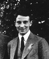
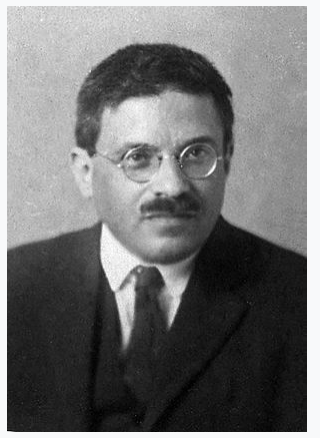
Oskar Klein (1894 – 1977)
Oskar Klein was a Swedish physicist who was in the “second wave” of quantum physicists just a few years behind the titans Heisenberg and Schrödinger and Pauli. He began as a student in physical chemistry working in Stockholm under the famous Arrhenius. It was arranged for him to work in France and Germany in 1914, but he was caught in Paris at the onset of World War I. Returning to Sweden, he enlisted in military service from 1915 to 1916 and then joined Arrhenius’ group at the Nobel Institute where he met Hendrick Kramers—Bohr’s direct assistant at Copenhagen at that time. At Kramer’s invitation, Klein traveled to Copenhagen and worked for a year with Kramers and Bohr before returning to defend his doctoral thesis in 1921 in the field of physical chemistry. Klein’s work with Bohr had opened his eyes to the possibilities of quantum theory, and he shifted his research interest away from physical chemistry. Unfortunately, there were no positions at that time in such a new field, so Klein accepted a position as assistant professor at the University of Michigan in Ann Arbor where he stayed from 1923 to 1925.
Oskar Klein in the late 1920’s
The Fifth Dimension
In an odd twist of fate, this isolation of Klein from the mainstream quantum theory being pursued in Europe freed him of the bandwagon effect and allowed him to range freely on topics of his own devising and certainly in directions all his own. Unaware of Kaluza’s previous work, Klein expanded Minkowski’s space-time from four to five spatial dimensions, just as Kaluza had done, but now with a quantum interpretation. This was not just an incremental step but had far-ranging consequences in the history of physics.
Klein found a way to keep the fifth dimension Euclidean in its metric properties while rolling itself up compactly into a cylinder with the radius of the Planck length—something inconceivably small. This compact fifth dimension made the manifold into something akin to an infinitesimal string. He published a short note in Nature magazine in 1926 on the possibility of identifying the electric charge within the 5-dimensional theory [Klein, 2916a]. He then returned to Sweden to take up a position at the University of Lund. This odd string-like feature of 5-dimensional space-time was picked up by Einstein and others in their search for unified field theories of physics, but the topic soon drifted from the lime light where it lay dormant for nearly fifty years until the first forays were made into string theory. String theory resurrected the Kaluza-Klein theory which has bourgeoned into the vast topic of String Theory today, including Superstrings that occur in 10+1 dimensionsat the frontiers of physics.
Dirac Electrons without the Spin: Klein-Gordon Equation
Once back in Europe, Klein reengaged with the mainstream trends in the rapidly developing quantum theory and in 1926 developed a relativistic quantum theory of the electron [Klein, 1926b]. Around the same time Walter Gordon also proposed this equation, which is now called the “Klein-Gordon Equation”. The equation was a classic wave equation that was second order in both space and time. This was the most natural form for a wave equation for quantum particles and Schrödinger himself had started with this form. But Schrödinger had quickly realized that the second-order time term in the equation did not capture the correct structure of the hydrogen atom, which led him to express the time-dependent term in first order and non-relativistically—which is today’s “Schrödinger Equation”. The problem was in the spin of the electron. The electron is a spin-1/2 particle, a Fermion, which has special transformation properties. It was Dirac a few years later who discovered how to express the relativistic wave equation for the electron—not by promoting the time-dependent term to second order, but by demoting the space-dependent term to first order. The first-order expression for both the space and time derivatives goes hand in hand with the Pauli spin matrices for the electron, and the Dirac Equation is the appropriate relativistically-correct wave equation for the electron.
Klein’s relativistic quantum wave equation does turn out to be the relevant form for a spin-less particle like the pion, but the pion decays by the strong nuclear force and the Klein-Gordon equation is not a practical description. However, the Higgs boson also is a spin-zero particle, and the Klein-Gordon expression does have relevance for this fundamental exchange particle.
Klein Tunneling
In those early days of the late 1920’s, the nature of the nucleus was still a mystery, especially the problem of nuclear radioactivity where a neutron could convert to a proton with the emission of an electron. Some suggested that the neutron was somehow a proton that had captured an electron in a potential barrier. Klein showed that this was impossible, that the electrons would be highly relativistic—something known as a Dirac electron—and they would tunnel with perfect probability through any potential barrier [Klein, 1929]. Therefore, Klein concluded, no nucleon or nucleus could bind an electron.
This phenomenon of unity transmission through a barrier became known as Klein tunneling. The relativistic electron transmits perfectly through an arbitrary potential barrier—independent of its width or height. This is unlike light that transmits through a dielectric slab in resonances that depend on the thickness of the slab—also known as a Fabry-Perot interferometer. The Dirac electron can have any energy, and the potential barrier can have any width, yet the electron will tunnel with 100% probability. How can this happen?
The answer has to do with the dispersion (velocity versus momentum) of the Dirac electron. As the momentum changes in a potential the speed of the Dirac electron stays constant. In the potential barrier, the moment flips sign, but the speed remains unchanged. This is equivalent to the effects of negative refractive index in optics. If a photon travels through a material with negative refractive index, its momentum is flipped, but its speed remains unchanged. From Fermat’s principle, it is speed which determines how a particle like a photon refracts, so if there is no speed change, then there is no reflection.
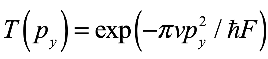
For the case of Dirac electrons in a potential with field F, speed v and transverse momentum py, the transmission coefficient is given by
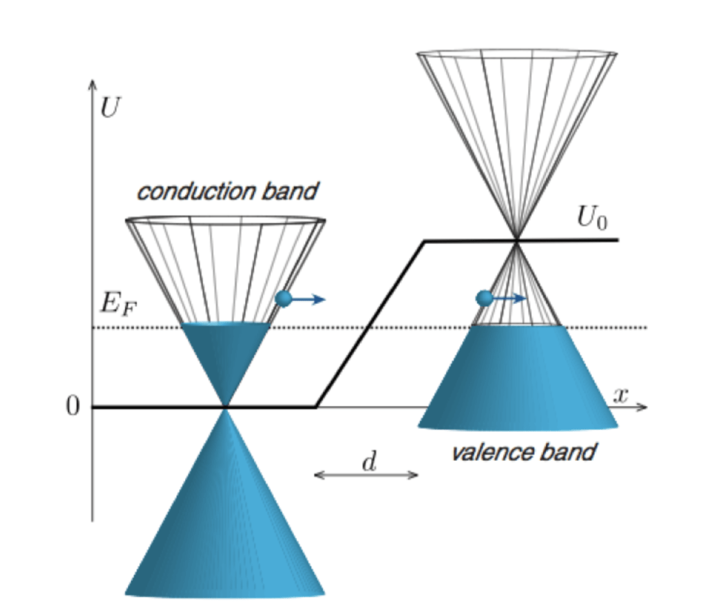
If the transverse momentum is zero, then the transmission is perfect. A visual schematic of the role of dispersion and potentials for Dirac electrons undergoing Klein tunneling is shown in the next figure.
In this case, even if the transverse momentum is not strictly zero, there can still be perfect transmission. It is simply a matter of matching speeds.
Graphene became famous over the past decade because its electron dispersion relation is just like a relativistic Dirac electron with a Dirac point between conduction and valence bands. Evidence for Klein tunneling in graphene systems has been growing, but clean demonstrations have remained difficult to observe.
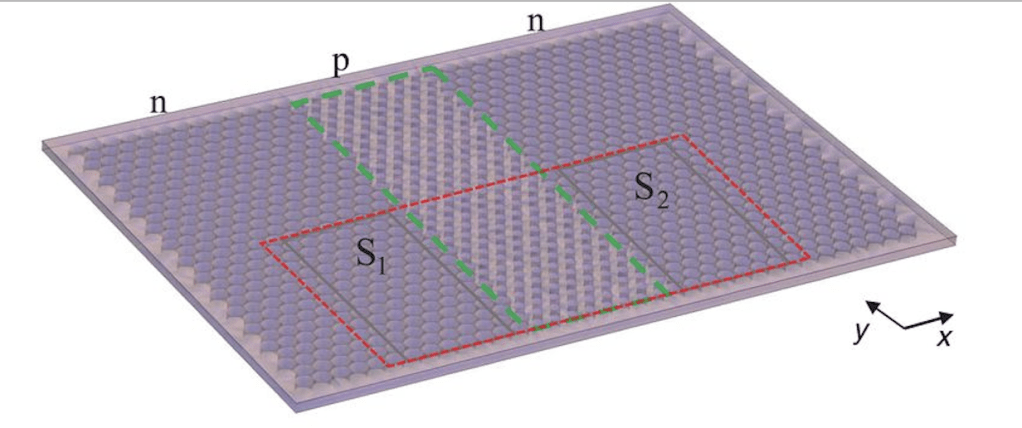
Now, published in the Dec. 2020 issue of Science magazine—almost a century after Klein first proposed it—an experimental group at the University of California at Berkeley reports a beautiful experimental demonstration of Klein tunneling—not from a nucleus, but in an acoustic honeycomb sounding board the size of a small table—making an experimental analogy between acoustics and Dirac electrons that bears out Klein’s theory.
In this special sounding board, it is not electrons but phonons—acoustic vibrations—that have a Dirac point. Furthermore, by changing the honeycomb pattern, the bands can be shifted, just like in a p-n-p junction, to produce a potential barrier. The Berkeley group, led by Xiang Zhang (now president of Hong Kong University), fabricated the sounding board that is about a half-meter in length, and demonstrated dramatic Klein tunneling.
It is amazing how long it can take between the time a theory is first proposed and the time a clean experimental demonstration is first performed. Nearly 90 years has elapsed since Klein first derived the phenomenon. Performing the experiment with actual relativistic electrons was prohibitive, but bringing the Dirac electron analog into the solid state has allowed the effect to be demonstrated easily.
References
[1921] Kaluza, Theodor (1921). “Zum Unitätsproblem in der Physik”. Sitzungsber. Preuss. Akad. Wiss. Berlin. (Math. Phys.): 966–972
[1926a] Klein, O. (1926). “The Atomicity of Electricity as a Quantum Theory Law”. Nature118: 516-516.
[1926b] Klein, O. (1926). “Quantentheorie und fünfdimensionale Relativitätstheorie”. Zeitschrift für Physik. 37 (12): 895
[1929] Klein, O. (1929). “Die Reflexion von Elektronen an einem Potentialsprung nach der relativistischen Dynamik von Dirac”. Zeitschrift für Physik. 53 (3–4): 157
The quantum of light—the photon—is a little over 100 years old. It was born in 1905 when Einstein merged Planck’s blackbody quantum hypothesis with statistical mechanics and concluded that light itself must be quantized. No one believed him! Fast forward to today, and the photon is a modern workhorse of modern quantum technology. Quantum encryption and communication are performed almost exclusively with photons, and many prototype quantum computers are optics based. Quantum optics also underpins atomic and molecular optics (AMO), which is one of the hottest and most rapidly advancing frontiers of physics today.
Only after the availability of “quantum” light sources … could photon numbers be manipulated at will, launching the modern era of quantum optics.
This blog tells the story of the early days of the photon and of quantum optics. It begins with Einstein in 1905 and ends with the demonstration of photon anti-bunching that was the first fundamentally quantum optical phenomenon observed seventy years later in 1977. Across that stretch of time, the photon went from a nascent idea in Einstein’s fertile brain to the most thoroughly investigated quantum particle in the realm of physics.
The Photon: Albert Einstein (1905)
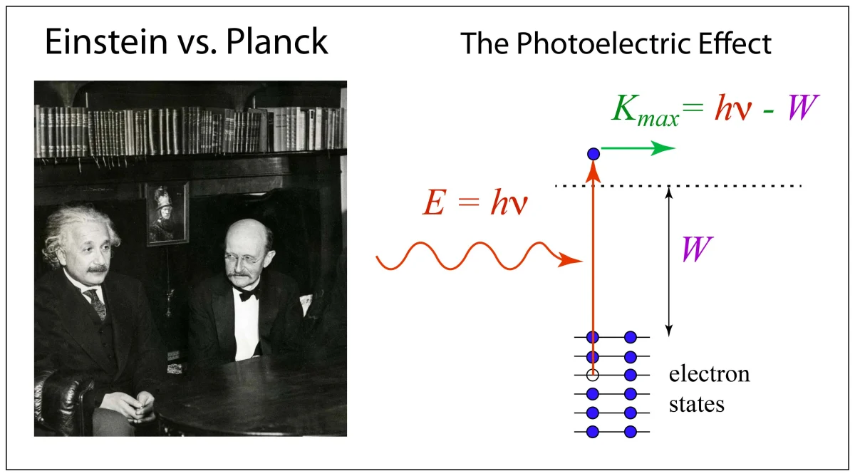
When Planck presented his quantum hypothesis in 1900 to the German Physical Society [1], his model of black body radiation retained all its classical properties but one—the quantized interaction of light with matter. He did not think yet in terms of quanta, only in terms of steps in a continuous interaction.
The quantum break came from Einstein when he published his 1905 paper proposing the existence of the photon—an actual quantum of light that carried with it energy and momentum [2]. His reasoning was simple and iron-clad, resting on Planck’s own blackbody relation that Einstein combined with simple reasoning from statistical mechanics. He was led inexorably to the existence of the photon. Unfortunately, almost no one believed him (see my blog on Einstein and Planck).
This was before wave-particle duality in quantum thinking, so the notion that light—so clearly a wave phenomenon—could be a particle was unthinkable. It had taken half of the 19th century to rid physics of Newton’s corpuscules and emmisionist theories of light, so to bring it back at the beginning of the 20th century seemed like a great blunder. However, Einstein persisted.
In 1909 he published a paper on the fluctuation properties of light [3] in which he proposed that the fluctuations observed in light intensity had two contributions: one from the discreteness of the photons (what we call “shot noise” today) and one from the fluctuations in the wave properties. Einstein was proposing that both particle and wave properties contributed to intensity fluctuations, exhibiting simultaneous particle-like and wave-like properties. This was one of the first expressions of wave-particle duality in modern physics.
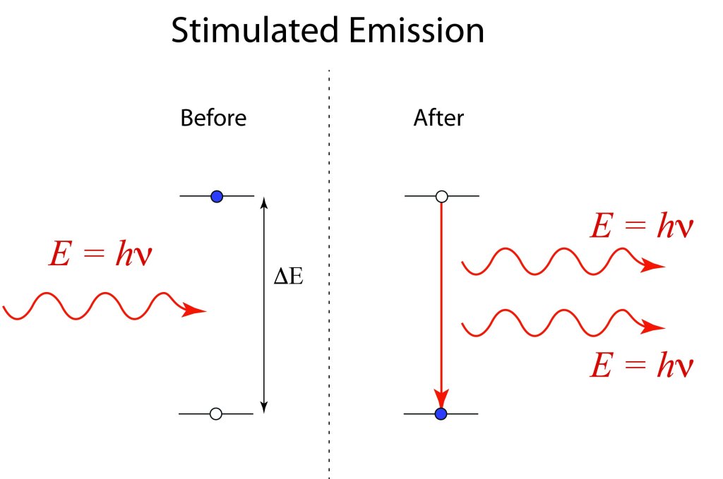
In 1916 and 1917 Einstein took another bold step and proposed the existence of stimulated emission [4]. Once again, his arguments were based on simple physics—this time the principle of detailed balance—and he was led to the audacious conclusion that one photon can stimulated the emission of another. This would become the basis of the laser forty-five years later.
While Einstein was confident in the reality of the photon, others sincerely doubted its existence. Robert Milliken (1868 – 1953) decided to put Einstein’s theory of photoelectron emission to the most stringent test ever performed. In 1915 he painstakingly acquired the definitive dataset with the goal to refute Einstein’s hypothesis, only to confirm it in spectacular fashion [5]. Partly based on Milliken’s confirmation of Einstein’s theory of the photon, Einstein was awarded the Nobel Prize in Physics in 1921.
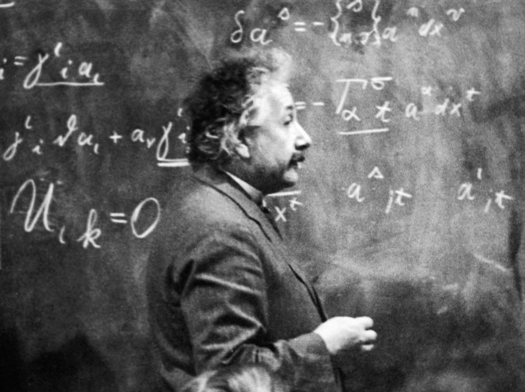
Einstein at a blackboard.
From that point onward, the physical existence of the photon was accepted and was incorporated routinely into other physical theories. Compton used the energy and the momentum of the photon in 1922 to predict and measure Compton scattering of x-rays off of electrons [6]. The photon was given its modern name by Gilbert Lewis in 1926 [7].
Single-Photon Interference: Geoffry Taylor (1909)
If a light beam is made up of a group of individual light quanta, then in the limit of very dim light, there should just be one photon passing through an optical system at a time. Therefore, to do optical experiments on single photons, one just needs to reach the ultimate dim limit. As simple and clear as this argument sounds, it has problems that only were sorted out after the Hanbury Brown and Twiss experiments in the 1950’s and the controversy they launched (see below). However, in 1909, this thinking seemed like a clear approach for looking for deviations in optical processes in the single-photon limit.
In 1909, Geoffry Ingram Taylor (1886 – 1975) was an undergraduate student at Cambridge University and performed a low-intensity Young’s double-slit experiment (encouraged by J. J. Thomson). At that time the idea of Einstein’s photon was only 4 years old, and Bohr’s theory of the hydrogen atom was still a year away. But Thomson believed that if photons were real, then their existence could possibly show up as deviations in experiments involving single photons. Young’s double-slit experiment is the classic demonstration of the classical wave nature of light, so performing it under conditions when (on average) only a single photon was in transit between a light source and a photographic plate seemed like the best place to look.
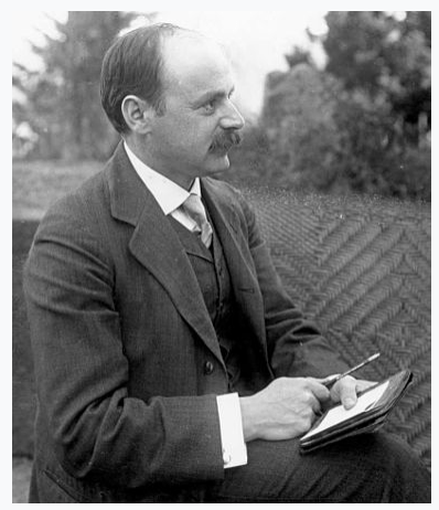
G. I. Taylor
The experiment was performed by finding an optimum exposure of photographic plates in a double slit experiment, then reducing the flux while increasing the exposure time, until the single-photon limit was achieved while retaining the same net exposure of the photographic plate. Under the lowest intensity, when only a single photon was in transit at a time (on average), Taylor performed the exposure for three months. To his disappointment, when he developed the film, there was no significant difference between high intensity and low intensity interference fringes [8]. If photons existed, then their quantized nature was not showing up in the low-intensity interference experiment.
The reason that there is no single-photon-limit deviation in the behavior of the Young double-slit experiment is because Young’s experiment only measures first-order coherence properties. The average over many single-photon detection events is described equally well either by classical waves or by quantum mechanics. Quantized effects in the Young experiment could only appear in fluctuations in the arrivals of photons, but in Taylor’s day there was no way to detect the arrival of single photons.
Quantum Theory of Radiation : Paul Dirac (1927)
After Paul Dirac (1902 – 1984) was awarded his doctorate from Cambridge in 1926, he received a stipend that sent him to work with Niels Bohr (1885 – 1962) in Copenhagen. His attention focused on the electromagnetic field and how it interacted with the quantized states of atoms. Although the electromagnetic field was the classical field of light, it was also the quantum field of Einstein’s photon, and he wondered how the quantized harmonic oscillators of the electromagnetic field could be generated by quantum wavefunctions acting as operators. He decided that, to generate a photon, the wavefunction must operate on a state that had no photons—the ground state of the electromagnetic field known as the vacuum state.
Dirac put these thoughts into their appropriate mathematical form and began work on two manuscripts. The first manuscript contained the theoretical details of the non-commuting electromagnetic field operators. He called the process of generating photons out of the vacuum “second quantization”. In second quantization, the classical field of electromagnetism is converted to an operator that generates quanta of the associated quantum field out of the vacuum (and also annihilates photons back into the vacuum). The creation operators can be applied again and again to build up an N-photon state containing N photons that obey Bose-Einstein statistics, as they must, as required by their integer spin, and agreeing with Planck’s blackbody radiation.
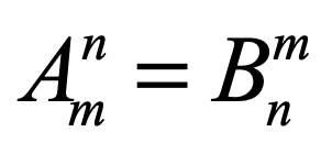
Dirac then showed how an interaction of the quantized electromagnetic field with quantized energy levels involved the annihilation and creation of photons as they promoted electrons to higher atomic energy levels, or demoted them through stimulated emission. Very significantly, Dirac’s new theory explained the spontaneous emission of light from an excited electron level as a direct physical process that creates a photon carrying away the energy as the electron falls to a lower energy level. Spontaneous emission had been explained first by Einstein more than ten years earlier when he derived the famous A and B coefficients [4], but the physical mechanism for these processes was inferred rather than derived. Dirac, in late 1926, had produced the first direct theory of photon exchange with matter [9].
Paul Dirac in his early days.
Einstein-Podolsky-Rosen (EPR) and Bohr (1935)
The famous dialog between Einstein and Bohr at the Solvay Conferences culminated in the now famous “EPR” paradox of 1935 when Einstein published (together with B. Podolsky and N. Rosen) a paper that contained a particularly simple and cunning thought experiment. In this paper, not only was quantum mechanics under attack, but so was the concept of reality itself, as reflected in the paper’s title “Can Quantum Mechanical Description of Physical Reality Be Considered Complete?” [10].
Bohr and Einstein at Paul Ehrenfest’s house in 1925.
Einstein considered an experiment on two quantum particles that had become “entangled” (meaning they interacted) at some time in the past, and then had flown off in opposite directions. By the time their properties are measured, the two particles are widely separated. Two observers each make measurements of certain properties of the particles. For instance, the first observer could choose to measure either the position or the momentum of one particle. The other observer likewise can choose to make either measurement on the second particle. Each measurement is made with perfect accuracy. The two observers then travel back to meet and compare their measurements. When the two experimentalists compare their data, they find perfect agreement in their values every time that they had chosen (unbeknownst to each other) to make the same measurement. This agreement occurred either when they both chose to measure position or both chose to measure momentum.
It would seem that the state of the particle prior to the second measurement was completely defined by the results of the first measurement. In other words, the state of the second particle is set into a definite state (using quantum-mechanical jargon, the state is said to “collapse”) the instant that the first measurement is made. This implies that there is instantaneous action at a distance −− violating everything that Einstein believed about reality (and violating the law that nothing can travel faster than the speed of light). He therefore had no choice but to consider this conclusion of instantaneous action to be false. Therefore quantum mechanics could not be a complete theory of physical reality −− some deeper theory, yet undiscovered, was needed to resolve the paradox.
Bohr, on the other hand, did not hold “reality” so sacred. In his rebuttal to the EPR paper, which he published six months later under the identical title [11], he rejected Einstein’s criterion for reality. He had no problem with the two observers making the same measurements and finding identical answers. Although one measurement may affect the conditions of the second despite their great distance, no information could be transmitted by this dual measurement process, and hence there was no violation of causality. Bohr’s mind-boggling viewpoint was that reality was nonlocal, meaning that in the quantum world the measurement at one location does influence what is measured somewhere else, even at great distance. Einstein, on the other hand, could not accept a nonlocal reality.
Entangled versus separable states. When the states are separable, no measurement on photon A has any relation to measurements on photon B. However, in the entangled case, all measurements on A are related to measurements on B (and vice versa) regardless of what decision is made to make what measurement on either photon, or whether the photons are separated by great distance. The entangled wave-function is “nonlocal” in the sense that it encompasses both particles at the same time, no matter how far apart they are.
The Intensity Interferometer: Hanbury Brown and Twiss (1956)
Optical physics was surprisingly dormant from the 1930’s through the 1940’s. Most of the research during this time was either on physical optics, like lenses and imaging systems, or on spectroscopy, which was more interested in the physical properties of the materials than in light itself. This hiatus from the photon was about to change dramatically, not driven by physicists, but driven by astronomers.
The development of radar technology during World War II enabled the new field of radio astronomy both with high-tech receivers and with a large cohort of scientists and engineers trained in radio technology. In the late 1940’s and early 1950’s radio astronomy was starting to work with long baselines to better resolve radio sources in the sky using interferometery. The first attempts used coherent references between two separated receivers to provide a common mixing signal to perform field-based detection. However, the stability of the reference was limiting, especially for longer baselines.
In 1950, a doctoral student in the radio astronomy department of the University of Manchester, R. Hanbury Brown, was given the task to design baselines that could work at longer distances to resolve smaller radio sources. After struggling with the technical difficulties of providing a coherent “local” oscillator for distant receivers, Hanbury Brown had a sudden epiphany one evening. Instead of trying to reference the field of one receiver to the field of another, what if, instead, one were to reference the intensity of one receiver to the intensity of the other, specifically correlating the noise on the intensity? To measure intensity requires no local oscillator or reference field. The size of an astronomical source would then show up in how well the intensity fluctuations correlated with each other as the distance between the receivers was changed. He did a back of the envelope calculation that gave him hope that his idea might work, but he needed more rigorous proof if he was to ask for money to try out his idea. He tracked down Richard Twiss at a defense research lab and the two working out the theory of intensity correlations for long-baseline radio interferometry. Using facilities at the famous Jodrell Bank Radio Observatory at Manchester, they demonstrated the principle of their intensity interferometer and measured the angular size of Cygnus A and Cassiopeia A, two of the strongest radio sources in the Northern sky.
R. Hanbury Brown
One of the surprising side benefits of the intensity interferometer over field-based interferometry was insensitivity to environmental phase fluctuations. For radio astronomy the biggest source of phase fluctuations was the ionosphere, and the new intensity interferometer was immune to its fluctuations. Phase fluctuations had also been the limiting factor for the Michelson stellar interferometer which had limited its use to only about half a dozen stars, so Hanbury Brown and Twiss decided to revisit visible stellar interferometry using their new concept of intensity interferometry.
To illustrate the principle for visible wavelengths, Hanbury Brown and Twiss performed a laboratory experiment to correlate intensity fluctuations in two receivers illuminated by a common source through a beam splitter. The intensity correlations were detected and measured as a function of path length change, illustrating an excess correlation in noise for short path lengths that decayed as the path length increased. They published their results in Nature magazine in 1956 that immediately ignited a firestorm of protest from physicists [12].
In the 1950’s, many physicists had embraced the discrete properties of the photon and had developed a misleading mental picture of photons as individual and indivisible particles that could only go one way or another from a beam splitter, but not both. Therefore, the argument went, if the photon in an attenuated beam was detected in one detector at the output of a beam splitter, then it cannot be detected at the other. This would produce an anticorrelation in coincidence counts at the two detectors. However, the Hanbury Brown Twiss (HBT) data showed a correlation from the two detectors. This launched an intense controversy in which some of those who accepted the results called for a radical new theory of the photon, while most others dismissed the HBT results as due to systematics in the light source. The heart of this controversy was quickly understood by the Nobel laureate E. M Purcell. He correctly pointed out that photons are bosons and are indistinguishable discrete particles and hence are likely to “bunch” together, according to quantum statistics, even under low light conditions [13]. Therefore, attenuated “chaotic” light would indeed show photodetector correlations, even if the average photon number was less than a single photon at a time, the photons would still bunch.
The bunching of photons in light is a second order effect that moves beyond the first-order interference effects of Young’s double slit, but even here the quantum nature of light is not required. A semiclassical theory of light emission from a spectral line with a natural bandwidth also predicts intensity correlations, and the correlations are precisely what would be observed for photon bunching. Therefore, even the second-order HBT results, when performed with natural light sources, do not distinguish between classical and quantum effects in the experimental results. But this reliance on natural light sources was about to change fundmaentally with the invention of the laser.
Invention of the Laser : Ted Maiman (1959)
One of the great scientific breakthroughs of the 20th century was the nearly simultaneous yet independent realization by several researchers around 1951 (by Charles H. Townes of Columbia University, by Joseph Weber of the University of Maryland, and by Alexander M. Prokhorov and Nikolai G. Basov at the Lebedev Institute in Moscow) that clever techniques and novel apparati could be used to produce collections of atoms that had more electrons in excited states than in ground states. Such a situation is called a population inversion. If this situation could be attained, then according to Einstein’s 1917 theory of photon emission, a single photon would stimulate a second photon, which in turn would stimulate two additional electrons to emit two identical photons to give a total of four photons −− and so on. Clearly this process turns a single photon into a host of photons, all with identical energy and phase.
Theodore Maiman
Charles Townes and his research group were the first to succeed in 1953 in producing a device based on ammonia molecules that could work as an intense source of coherent photons. The initial device did not amplify visible light, but amplified microwave photons that had wavelengths of about 3 centimeters. They called the process microwave amplification by stimulated emission of radiation, hence the acronym “MASER”. Despite the significant breakthrough that this invention represented, the devices were very expensive and difficult to operate. The maser did not revolutionize technology, and some even quipped that the acronym stood for “Means of Acquiring Support for Expensive Research”. The maser did, however, launch a new field of study, called quantum electronics, that was the direct descendant of Einstein’s 1917 paper. Most importantly, the existence and development of the maser became the starting point for a device that could do the same thing for light.
The race to develop an optical maser (later to be called laser, for light amplification by stimulated emission of radiation) was intense. Many groups actively pursued this holy grail of quantum electronics. Most believed that it was possible, which made its invention merely a matter of time and effort. This race was won by Theodore H. Maiman at Hughes Research Laboratory in Malibu California in 1960 [14]. He used a ruby crystal that was excited into a population inversion by an intense flash tube (like a flash bulb) that had originally been invented for flash photography. His approach was amazingly simple −− blast the ruby with a high-intensity pulse of light and see what comes out −− which explains why he was the first. Most other groups had been pursuing much more difficult routes because they believed that laser action would be difficult to achieve.
Perhaps the most important aspect of Maiman’s discovery was that it demonstrated that laser action was actually much simpler than people anticipated, and that laser action is a fairly common phenomenon. His discovery was quickly repeated by other groups, and then additional laser media were discovered such as helium-neon gas mixtures, argon gas, carbon dioxide gas, garnet lasers and others. Within several years, over a dozen different material and gas systems were made to lase, opening up wide new areas of research and development that continues unabated to this day. It also called for new theories of optical coherence to explain how coherent laser light interacted with matter.
Coherent States : Glauber (1963)
The HBT experiment had been performed with attenuated chaotic light that had residual coherence caused by the finite linewidth of the filtered light source. The theory of intensity correlations for this type of light was developed in the 1950’s by Emil Wolf and Leonard Mandel using a semiclassical theory in which the statistical properties of the light was based on electromagnetics without a direct need for quantized photons. The HBT results were fully consistent with this semiclassical theory. However, after the invention of the laser, new “coherent” light sources became available that required a fundamentally quantum depiction.
Roy Glauber was a theoretical physicist who received his PhD working with Julian Schwinger at Harvard. He spent several years as a post-doc at Princeton’s Institute for Advanced Study starting in 1949 at the time when quantum field theory was being developed by Schwinger, Feynman and Dyson. While Feynman was off in Brazil for a year learning to play the bongo drums, Glauber filled in for his lectures at Cal Tech. He returned to Harvard in 1952 in the position of an assistant professor. He was already thinking about the quantum aspects of photons in 1956 when news of the photon correlations in the HBT experiment were published, and when the laser was invented three years later, he began developing a theory of photon correlations in laser light that he suspected would be fundamentally different than in natural chaotic light.
Roy Glauber
Because of his background in quantum field theory, and especially quantum electrodynamics, it was a fairly easy task to couch the quantum optical properties of coherent light in terms of Dirac’s creation and annihilation operators of the electromagnetic field. Related to the minimum-uncertainty wave functions derived initially by Schrödinger in the late 1920’s, Glauber developed a “coherent state” operator that was a minimum uncertainty state of the quantized electromagnetic field [15]. This coherent state represents a laser operating well above the lasing threshold and predicted that the HBT correlations would vanish. Glauber was awarded the Nobel Prize in Physics in 2005 for his work on such “Glauber” states in quantum optics.
Single-Photon Optics: Kimble and Mandel (1977)
Beyond introducing coherent states, Glauber’s new theoretical approach, and parallel work by George Sudarshan around the same time [16], provided a new formalism for exploring quantum optical properties in which fundamentally quantum processes could be explored that could not be predicted using only semiclassical theory. For instance, one could envision producing photon states in which the photon arrivals at a detector could display the kind of anti-bunching that had originally been assumed (in error) by the critics of the HBT experiment. A truly one-photon state, also known as a Fock state or a number state, would be the extreme limit in which the quantum field possessed a single quantum that could be directed at a beam splitter and would emerge either from one side or the other with complete anti-correlation. However, generating such a state in the laboratory remained a challenge.
In 1975 by Carmichel and Walls predicted that resonance fluorescence could produce quantized fields that had lower correlations than coherent states [17]. In 1977 H. J. Kimble, M. Dagenais and L. Mandel demonstrated, for the first time, photon antibunching between two photodetectors at the two ports of a beam splitter [18]. They used a beam of sodium atoms pumped by a dye laser.
This first demonstration of photon antibunching represents a major milestone in the history of quantum optics. Taylor’s first-order experiments in 1909 showed no difference between classical electromagnetic waves and a flux of photons. Similarly the second-order HBT experiment of 1956 using chaotic light could be explained equally well using classical or quantum approaches to explain the observed photon correlations. Even laser light (when the laser is operated far above threshold) produced classic “classical” wave effects with only the shot noise demonstrating the discreteness of photon arrivals. Only after the availability of “quantum” light sources, beginning with the work of Kimble and Mandel, could photon numbers be manipulated at will, launching the modern era of quantum optics. Later experiments by them and others have continually improved the control of photon states.
By David D. Nolte, Jan. 18, 2021
TimeLine:
1900 – Planck (1901). “Law of energy distribution in normal spectra.” Annalen Der Physik 4(3): 553-563.
1905 – A. Einstein (1905). “Generation and conversion of light with regard to a heuristic point of view.” Annalen Der Physik 17(6): 132-148.
1909 – A. Einstein (1909). “On the current state of radiation problems.” Physikalische Zeitschrift 10: 185-193.
1909 – G.I. Taylor: Proc. Cam. Phil. Soc. Math. Phys. Sci. 15 , 114 (1909) Single photon double-slit experiment
1915 – Millikan, R. A. (1916). “A direct photoelectric determination of planck’s “h.”.” Physical Review 7(3): 0355-0388. Photoelectric effect.
1916 – Einstein, A. (1916). “Strahlungs-Emission un -Absorption nach der Quantentheorie.” Verh. Deutsch. Phys. Ges. 18: 318.. Einstein predicts stimulated emission
1923 –Compton, Arthur H. (May 1923). “A Quantum Theory of the Scattering of X-Rays by Light Elements”. Physical Review. 21 (5): 483–502.
1926 – Lewis, G. N. (1926). “The conservation of photons.” Nature 118: 874-875.. Gilbert Lewis named “photon”
1927 – D. Dirac, P. A. M. (1927). “The quantum theory of the emission and absorption of radiation.” Proceedings of the Royal Society of London Series a-Containing Papers of a Mathematical and Physical Character 114(767): 243-265.
1932 – E. P. Wigner: Phys. Rev. 40, 749 (1932)
1935 – A. Einstein, B. Podolsky, N. Rosen: Phys. Rev. 47 , 777 (1935). EPR paradox.
1935 – N. Bohr: Phys. Rev. 48 , 696 (1935). Bohr’s response to the EPR paradox.
1963 – R. J. Glauber: Phys. Rev. 130 , 2529 (1963) Coherent states
1963 – E. C. G. Sudarshan: Phys. Rev. Lett. 10, 277 (1963) Coherent states
1964 – P. L. Kelley, W.H. Kleiner: Phys. Rev. 136 , 316 (1964)
1966 – F. T. Arecchi, E. Gatti, A. Sona: Phys. Rev. Lett. 20 , 27 (1966); F.T. Arecchi, Phys. Lett. 16 , 32 (1966)
1966 – J. S. Bell: Physics 1 , 105 (1964); Rev. Mod. Phys. 38 , 447 (1966) Bell inequalities
1967 – R. F. Pfleegor, L. Mandel: Phys. Rev. 159 , 1084 (1967) Interference at single photon level
1967 – M. O. Scully, W.E. Lamb: Phys. Rev. 159 , 208 (1967). Quantum theory of laser
1967 – B. R. Mollow, R. J. Glauber: Phys. Rev. 160, 1097 (1967); 162, 1256 (1967) Parametric converter
1969 – M. O. Scully, W.E. Lamb: Phys. Rev. 179 , 368 (1969). Quantum theory of laser
1969 – M. Lax, W.H. Louisell: Phys. Rev. 185 , 568 (1969). Quantum theory of laser
1975 – Carmichael, H. J. and D. F. Walls (1975). Journal of Physics B-Atomic Molecular and Optical Physics 8(6): L77-L81. Photon anti-bunching predicted in resonance fluorescence
1977 – H. J. Kimble, M. Dagenais and L. Mandel (1977) Photon antibunching in resonance fluorescence. Phys. Rev. Lett. 39, 691-5: Kimble, Dagenais and Mandel demonstrate the effect of antibunching
[4] Einstein, A. (1916). “Strahlungs-Emission un -Absorption nach der Quantentheorie.” Verh. Deutsch. Phys. Ges. 18: 318; Einstein, A. (1917). “Quantum theory of radiation.” Physikalische Zeitschrift 18: 121-128.
[10] Einstein, A., B. Podolsky and N. Rosen (1935). “Can quantum-mechanical description of physical reality be considered complete?” Physical Review 47(10): 0777-0780.
[12] Brown, R. H. and R. Q. Twiss (1956). “Correlation Between Photons in 2 Coherent Beams of Light.” Nature177(4497): 27-29; [1] R. H. Brown and R. Q. Twiss, “Test of a new type of stellar interferometer on Sirius,” Nature, vol. 178, no. 4541, pp. 1046-1048, (1956).
[15] Glauber, R. J. (1963). “Photon Correlations.” Physical Review Letters 10(3): 84.
[16] Sudarshan, E. C. G. (1963). “Equivalence of semiclassical and quantum mechanical descriptions of statistical light beams.” Physical Review Letters 10(7): 277-&.; Mehta, C. L. and E. C. Sudarshan (1965). “Relation between quantum and semiclassical description of optical coherence.” Physical Review 138(1B): B274.
[17] Carmichael, H. J. and D. F. Walls (1975). “Quantum treatment of spontaneous emission from a strongly driven 2-level atom.” Journal of Physics B-Atomic Molecular and Optical Physics 8(6): L77-L81.
Quantum sensors have amazing powers. They can detect the presence of an obstacle without ever interacting with it. For instance, consider a bomb that is coated with a light sensitive layer that sets off the bomb if it absorbs just a single photon. Then put this bomb inside a quantum sensor system and shoot photons at it. Remarkably, using the weirdness of quantum mechanics, it is possible to design the system in such a way that you can detect the presence of the bomb using photons without ever setting it off. How can photons see the bomb without illuminating it? The answer is a bizarre side effect of quantum physics in which quantum wavefunctions are recognized as the root of reality as opposed to the pesky wavefunction collapse at the moment of measurement.
The ability for a quantum system to see an object with light, without exposing it, is uniquely a quantum phenomenon that has no classical analog.
All Paths Lead to Feynman
When Richard Feynman was working on his PhD under John Archibald Wheeler at Princeton in the early 1940’s he came across an obscure paper written by Paul Dirac in 1933 that connected quantum physics with classical Lagrangian physics. Dirac had recognized that the phase of a quantum wavefunction was analogous to the classical quantity called the “Action” that arises from Lagrangian physics. Building on this concept, Feynman constructed a new interpretation of quantum physics, known as the “many histories” interpretation, that occupies the middle ground between Schrödinger’s wave mechanics and Heisenberg’s matrix mechanics. One of the striking consequences of the many histories approach is the emergence of the principle of least action—a classical concept—into interpretations of quantum phenomena. In this approach, Feynman considered ALL possible histories for the propagation of a quantum particle from one point to another, he tabulated the quantum action in the phase factor, and he then summed all of these histories.
One of the simplest consequences of the sum over histories is a quantum interpretation of Snell’s law of refraction in optics. When summing over all possible trajectories of a photon from a point above to a point below an interface, there are a subset of paths for which the action integral varies very little from one path in the subset to another. The consequence of this is that the phases of all these paths add constructively, producing a large amplitude to the quantum wavefunction along the centroid of these trajectories. Conversely, for paths far away from this subset, the action integral takes on many values and the phases tend to interfere destructively, canceling the wavefunction along these other paths. Therefore, the most likely path of the photon between the two points is the path of maximum constructive interference and hence the path of stationary action. It is simple so show that this path is none other than the classical path determined by Snell’s Law and equivalently by Fermat’s principle of least time. With the many histories approach, we can add the principle of least (or stationary) action to the list of explanations of Snell’s Law. This argument holds as well for an electron (with mass and a de Broglie wavelength) as it does for a photon, so this not just a coincidence specific to optics but is a fundamental part of quantum physics.
A more subtle consequence of the sum over histories view of quantum phenomena is Young’s double slit experiment for electrons, shown at the top of Fig 1. The experiment consists of a source that emits only a single electron at a time that passes through a double-slit mask to impinge on an electron detection screen. The wavefunction for a single electron extends continuously throughout the full spatial extent of the apparatus, passing through both slits. When the two paths intersect at the screen, the difference in the quantum phases of the two paths causes the combined wavefunction to have regions of total constructive interference and other regions of total destructive interference. The probability of detecting an electron is proportional to the squared amplitude of the wavefunction, producing a pattern of bright stripes separated by darkness. At positions of destructive interference, no electrons are detected when both slits are open. However, if an opaque plate blocks the upper slit, then the interference pattern disappears, and electrons can be detected at those previously dark locations. Therefore, the presence of the object can be deduced by the detection of electrons at locations that should be dark.
Fig. 1 Demonstration of the sum over histories in a double-slit experiment for electrons. In the upper frame, the electron interference pattern on the phosphorescent screen produces bright and dark stripes. No electrons hit the screen in a dark stripe. When the upper slit is blocked (bottom frame), the interference pattern disappears, and an electron can arrive at the location that had previously been dark.
Consider now when the opaque plate is an electron-sensitive detector. In this case, a single electron emitted by the source can be detected at the screen or at the plate. If it is detected at the screen, it can appear at the location of a dark fringe, heralding the presence of the opaque plate. Yet the quantum conundrum is that when the electron arrives at a dark fringe, it must be detected there as a whole, it cannot be detected at the electron-sensitive plate too. So how does the electron sense the presence of the detector without exposing it, without setting it off?
In Feynman’s view, the electron does set off the detector as one possible history. And that history interferes with the other possible history when the electron arrives at the screen. While that interpretation may seem weird, mathematically it is a simple statement that the plate blocks the wavefunction from passing through the upper slit, so the wavefunction in front of the screen, resulting from all possible paths, has no interference fringes (other than possible diffraction from the lower slit). From this point of view, the wavefunction samples all of space, including the opaque plate, and the eventual absorption of a photon one place or another has no effect on the wavefunction. In this sense, it is the wavefunction, prior to any detection event, that samples reality. If the single electron happens to show up at a dark fringe at the screen, the plate, through its effects on the total wavefunction, has been detected without interacting with the photon.
This phenomenon is known as an interaction-free measurement, but there are definitely some semantics issues here. Just because the plate doesn’t absorb a photon, it doesn’t mean that the plate plays no role. The plate certainly blocks the wavefunction from passing through the upper slit. This might be called an “interaction”, but that phrase it better reserved for when the photon is actually absorbed, while the role of the plate in shaping the wavefunction is better described as one of the possible histories.
Quantum Seeing in the Dark
Although Feynman was thinking hard (and clearly) about these issues as he presented his famous lectures in physics at Cal Tech during 1961 to 1963, the specific possibility of interaction-free measurement dates more recently to 1993 when Avshalom C. Elitzur and Lev Vaidman at Tel Aviv University suggested a simple Michelson interferometer configuration that could detect an object half of the time without interacting with it [1]. They are the ones who first pressed this point home by thinking of a light-sensitive bomb. There is no mistaking when a bomb goes off, so it tends to give an exaggerated demonstration of the interaction-free measurement.
The Michelson interferometer for interaction-free measurement is shown in Fig. 2. This configuration uses a half-silvered beamsplitter to split the possible photon paths. When photons hit the beamsplitter, they either continue traveling to the right, or are deflected upwards. After reflecting off the mirrors, the photons again encounter the beamsplitter, where, in each case, they continue undeflected or are reflected. The result is that two paths combine at the beamsplitter to travel to the detector, while two other paths combine to travel back along the direction of the incident beam.
Fig. 2 A quantum-seeing in the dark (QSD) detector with a photo-sensitive bomb. A single photon is sent into the interferometer at a time. If the bomb is NOT present, destructive interference at the detector guarantees that the photon is not detected. However, if the bomb IS present, it destroys the destructive interference and the photon can arrive at the detector. That photon heralds the presence of the bomb without setting it off. (Reprinted from Mind @ Light Speed)
The paths of the light beams can be adjusted so that the beams that combine to travel to the detector experience perfect destructive interference. In this situation, the detector never detects light, and all the light returns back along the direction of the incident beam. Quantum mechanically, when only a single photon is present in the interferometer at a time, we would say that the quantum wavefunction of the photon interferes destructively along the path to the detector, and constructively along the path opposite to the incident beam, and the detector would detect no photons. It is clear that the unobstructed path of both beams results in the detector making no detections.
Now place the light sensitive bomb in the upper path. Because this path is no longer available to the photon wavefunction, the destructive interference of the wavefunction along the detector path is removed. Now when a single photon is sent into the interferometer, three possible things can happen. One, the photon is reflected by the beamsplitter and detonates the bomb. Two, the photon is transmitted by the beamsplitter, reflects off the right mirror, and is transmitted again by the beamsplitter to travel back down the incident path without being detected by the detector. Three, the photon is transmitted by the beamsplitter, reflects off the right mirror, and is reflected off the beamsplitter to be detected by the detector.
In this third case, the photon is detected AND the bomb does NOT go off, which succeeds at quantum seeing in the dark. The odds are much better than for Young’s experiment. If the bomb is present, it will detonate a maximum of 50% of the time. The other 50%, you will either detect a photon (signifying the presence of the bomb), or else you will not detect a photon (giving an ambiguous answer and requiring you to perform the experiment again). When you perform the experiment again, you again have a 50% chance of detonating the bomb, and a 25% chance of detecting it without it detonating, but again a 25% chance of not detecting it, and so forth. All in all, every time you send in a photon, you have one chance in four of seeing the bomb without detonating it. These are much better odds than for the Young’s apparatus where only exact detection of the photon at a forbidden location would signify the presence of the bomb.
It is possible to increase your odds above one chance in four by decreasing the reflectivity of the beamsplitter. In practice, this is easy to do simply by depositing less and less aluminum on the surface of the glass plate. When the reflectivity gets very low, let us say at the level of 1%, then most of the time the photon just travels back along the direction it came and you have an ambiguous result. On the other hand, when the photon does not return, there is an equal probability of detonation as detection. This means that, though you may send in many photons, your odds for eventually seeing the bomb without detonating it are nearly 50%, which is a factor of two better odds than for the half-silvered beamsplitter. A version of this experiment was performed by Paul Kwiat in 1995 as a postdoc at Innsbruck with Anton Zeilinger. It was Kwiat who coined the phrase “quantum seeing in the dark” as a catchier version of “interaction-free measurement” [2].
A 50% chance of detecting the bomb without setting it off sounds amazing, until you think that there is a 50% chance that it will go off and kill you. Then those odds don’t look so good. But optical phenomena never fail to surprise, and they never let you down. A crucial set of missing elements in the simple Michelson experiment was polarization-control using polarizing beamsplitters and polarization rotators. These are common elements in many optical systems, and when they are added to the Michelson quantum sensor, they can give almost a 100% chance of detecting the bomb without setting it off using the quantum Zeno effect.
The Quantum Zeno Effect
Photons carry polarization as their prime quantum number, with two possible orientations. These can be defined in different ways, but the two possible polarizations are orthogonal to each other. For instance, these polarization pairs can be vertical (V) and horizontal (H), or they can be right circular and left circular. One of the principles of quantum state evolution is that a quantum wavefunction can be maintained in a specific state, even if it has a tendency naturally to drift out of that state, by repeatedly making a quantum measurement that seeks to measure deviations from that state. In practice, the polarization of a photon can be maintained by repeatedly passing it through a polarizing beamsplitter with the polarization direction parallel to the original polarization of the photon. If there is a deviation in the photon polarization direction by a small angle, then a detector on the side port of the polarizing beamsplitter will fire with a probability equal to the square of the sine of the deviation. If the deviation angle is very small, say Δθ, then the probability of measuring the deviation is proportional to (Δθ)2, which is an even smaller number. Furthermore, the probability that the photon will transmit through the polarizing beamsplitter is equal to 1-(Δθ)2, which is nearly 100%.
This is what happens in Fig. 3 when the photo-sensitive bomb IS present. A single H-polarized photon is injected through a switchable mirror into the interferometer on the right. In the path of the photon is a polarization rotator that rotates the polarization by a small angle Δθ. There is nearly a 100% chance that the photon will transmit through the polarizing beamsplitter with perfect H-polarization reflect from the mirror and return through the polarizing beamsplitter, again with perfect H-polarization to pass through the polarization rotator to the switchable mirror where it reflects, gains another increment to its polarization angle, which is still small, and transmits through the beamsplitter, etc. At each pass, the photon polarization is repeatedly “measured” to be horizontal. After a number of passes N = π/Δθ/2, the photon is switched out of the interferometer and is transmitted through the external polarizing beamsplitter where it is detected at the H-photon detector.
Now consider what happens when the bomb IS NOT present. This time, even though there is a high amplitude for the transmitted photon, there is that Δθ amplitude for reflection out the V port. This small V-amplitude, when it reflects from the mirror, recombines with the H-amplitude at the polarizing beamsplitter to produce a polarization that has the same tilted polarizaton that it started with, sending it back in the direction from which it came. (In this situation, the detector on the “dark” port of the internal beamsplitter never sees the photon because of destructive interference along this path.) The photon is then rotated once more by the polarization rotator, and the photon polarization is rotated again, etc.. Now, after a number of passes N = π/Δθ/2, the photon has acquired a V polarization and is switched out of the interferometer. At the external polarizing beamsplitter it is reflected out of the V-port where it is detected at the V-photon detector.
Fig. 3 Quantum Zeno effect for interaction-free measurement. If the bomb is present, the H-photon detector detects the output photon without setting it off. The switchable mirror ejects the photon after it makes π/Δθ/2 round trips in the polarizing interferometer.
The two end results of this thought experiment are absolutely distinct, giving a clear answer to the question whether the bomb is present or not. If the bomb IS present, the H-detector fires. If the bomb IS NOT present, then the V-detector fires. Through all of this, the chance to set off the bomb is almost zero. Therefore, this quantum Zeno interaction-free measurement detects the bomb with nearly 100% efficiency with almost no chance of setting it off. This is the amazing consequence of quantum physics. The wavefunction is affected by the presence of the bomb, altering the interference effects that allow the polarization to rotate. But the likelihood of a photon being detected by the bomb is very low.
On a side note: Although ultrafast switchable mirrors do exist, the experiment was much easier to perform by creating a helix in the optical path through the system so that there is only a finite number of bounces of the photon inside the cavity. See Ref. [2] for details.
In conclusion, the ability for a quantum system to see an object with light, without exposing it, is uniquely a quantum phenomenon that has no classical analog. No E&M wave description can explain this effect.
Further Reading
I first wrote about quantum seeing the dark in my 2001 book on the future of optical physics and technology: Nolte, D. D. (2001). Mind at Light Speed : A new kind of intelligence. (New York, Free Press)
More on the story of Feynman and Wheeler and what they were trying to accomplish is told in Chapter 8 of Galileo Unbound on the physics and history of dynamics: Nolte, D. D. (2018). Galileo Unbound: A Path Across Life, the Universe and Everything (Oxford University Press).
Paul Kwiat introduced to the world to interaction-free measurements in 1995 in this illuminating Scientific American article: Kwiat, P., H. Weinfurter and A. Zeilinger (1996). “Quantum seeing in the dark – Quantum optics demonstrates the existence of interaction-free measurements: the detection of objects without light-or anything else-ever hitting them.” Scientific American 275(5): 72-78.
References
[1] Elitzur, A. C. and L. Vaidman (1993). “QUANTUM-MECHANICAL INTERACTION-FREE MEASUREMENTS.” Foundations of Physics 23(7): 987-997.
[2] Kwiat, P., H. Weinfurter, T. Herzog, A. Zeilinger and M. A. Kasevich (1995). “INTERACTION-FREE MEASUREMENT.” Physical Review Letters 74(24): 4763-4766.
Einstein is the alpha of the quantum. Einstein is also the omega. Although he was the one who established the quantum of energy and matter (see my Blog Einstein vs Planck), Einstein pitted himself in a running debate against Niels Bohr’s emerging interpretation of quantum physics that had, in Einstein’s opinion, severe deficiencies. Between sessions during a series of conferences known as the Solvay Congresses over a period of eight years from 1927 to 1935, Einstein constructed a challenges of increasing sophistication to confront Bohr and his quasi-voodoo attitudes about wave-function collapse. To meet the challenge, Bohr sharpened his arguments and bested Einstein, who ultimately withdrew from the field of battle. Einstein, as quantum physics’ harshest critic, played a pivotal role, almost against his will, establishing the Copenhagen interpretation of quantum physics that rules to this day, and also inventing the principle of entanglement which lies at the core of almost all quantum information technology today.
Debate Timeline
Fifth Solvay Congress: 1927 October Brussels: Debate Round 1
Einstein and ensembles
Sixth Solvay Congress: 1930 Debate Round 2
Photon in a box
Seventh Solvay Congress: 1933
Einstein absent (visiting the US when Hitler takes power…decides not to return to Germany.)
Physical Review 1935: Debate Round 3
EPR paper and Bohr’s response
Schrödinger’s Cat
Notable Nobel Prizes
1918 Planck
1921 Einstein
1922 Bohr
1932 Heisenberg
1933 Dirac and Schrödinger
The Solvay Conferences
The Solvay congresses were unparalleled scientific meetings of their day. They were attended by invitation only, and invitations were offered only to the top physicists concerned with the selected topic of each meeting. The Solvay congresses were held about every three years always in Belgium, supported by the Belgian chemical industrialist Ernest Solvay. The first meeting, held in 1911, was on the topic of radiation and quanta.
Fig. 1 First Solvay Congress (1911). Einstein (standing second from right) was one of the youngest attendees.
The fifth meeting, held in 1927, was on electrons and photons and focused on the recent rapid advances in quantum theory. The old quantum guard was invited—Planck, Bohr and Einstein. The new quantum guard was invited as well—Heisenberg, de Broglie, Schrödinger, Born, Pauli, and Dirac. Heisenberg and Bohr joined forces to present a united front meant to solidify what later became known as the Copenhagen interpretation of quantum physics. The basic principles of the interpretation include the wavefunction of Schrödinger, the probabilistic interpretation of Born, the uncertainty principle of Heisenberg, the complementarity principle of Bohr and the collapse of the wavefunction during measurement. The chief conclusion that Heisenberg and Bohr sought to impress on the assembled attendees was that the theory of quantum processes was complete, meaning that unknown or uncertain characteristics of measurements could not be attributed to lack of knowledge or understanding, but were fundamental and permanently inaccessible.
Fig. 2 Fifth Solvay Congress (1927). Einstein front and center. Bohr on the far right middle row.
Einstein was not convinced with that argument, and he rose to his feet to object after Bohr’s informal presentation of his complementarity principle. Einstein insisted that uncertainties in measurement were not fundamental, but were caused by incomplete information, that , if known, would accurately account for the measurement results. Bohr was not prepared for Einstein’s critique and brushed it off, but what ensued in the dining hall and the hallways of the Hotel Metropole in Brussels over the next several days has become one of the most famous scientific debates of the modern era, known as the Bohr-Einstein debate on the meaning of quantum theory. The debate gently raged night and day through the fifth congress, and was renewed three years later at the 1930 congress. It finished, in a final flurry of published papers in 1935 that launched some of the central concepts of quantum theory, including the idea of quantum entanglement and, of course, Schrödinger’s cat.
Einstein’s strategy, to refute Bohr, was to construct careful thought experiments that envisioned perfect experiments, without errors, that measured properties of ideal quantum systems. His aim was to paint Bohr into a corner from which he could not escape, caught by what Einstein assumed was the inconsistency of complementarity. Einstein’s “thought experiments” used electrons passing through slits, diffracting as required by Schrödinger’s theory, but being detected by classical measurements. Einstein would present a thought experiment to Bohr, who would then retreat to consider the way around Einstein’s arguments, returning the next hour or the next day with his answer, only to be confronted by yet another clever device of Einstein’s clever imagination that would force Bohr to retreat again. The spirit of this back and forth encounter between Bohr and Einstein is caught dramatically in the words of Paul Ehrenfest who witnessed the debate first hand, partially mediating between Bohr and Einstein, both of whom he respected deeply.
“Brussels-Solvay was fine!… BOHR towering over everybody. At first not understood at all … , then step by step defeating everybody. Naturally, once again the awful Bohr incantation terminology. Impossible for anyone else to summarise … (Every night at 1 a.m., Bohr came into my room just to say ONE SINGLE WORD to me, until three a.m.) It was delightful for me to be present during the conversation between Bohr and Einstein. Like a game of chess, Einstein all the time with new examples. In a certain sense a sort of Perpetuum Mobile of the second kind to break the UNCERTAINTY RELATION. Bohr from out of philosophical smoke clouds constantly searching for the tools to crush one example after the other. Einstein like a jack-in-the-box; jumping out fresh every morning. Oh, that was priceless. But I am almost without reservation pro Bohr and contra Einstein. His attitude to Bohr is now exacly like the attitude of the defenders of absolute simultaneity towards him …” [1]
The most difficult example that Einstein constructed during the fifth Solvary Congress involved an electron double-slit apparatus that could measure, in principle, the momentum imparted to the slit by the passing electron, as shown in Fig.3. The electron gun is a point source that emits the electrons in a range of angles that illuminates the two slits. The slits are small relative to a de Broglie wavelength, so the electron wavefunctions diffract according to Schrödinger’s wave mechanics to illuminate the detection plate. Because of the interference of the electron waves from the two slits, electrons are detected clustered in intense fringes separated by dark fringes.
So far, everyone was in agreement with these suggested results. The key next step is the assumption that the electron gun emits only a single electron at a time, so that only one electron is present in the system at any given time. Furthermore, the screen with the double slit is suspended on a spring, and the position of the screen is measured with complete accuracy by a displacement meter. When the single electron passes through the entire system, it imparts a momentum kick to the screen, which is measured by the meter. It is also detected at a specific location on the detection plate. Knowing the position of the electron detection, and the momentum kick to the screen, provides information about which slit the electron passed through, and gives simultaneous position and momentum values to the electron that have no uncertainty, apparently rebutting the uncertainty principle.
Fig. 3 Einstein’s single-electron thought experiment in which the recoil of the screen holding the slits can be measured to tell which way the electron went. Bohr showed that the more “which way” information is obtained, the more washed-out the interference pattern becomes.
This challenge by Einstein was the culmination of successively more sophisticated examples that he had to pose to combat Bohr, and Bohr was not going to let it pass unanswered. With ingenious insight, Bohr recognized that the key element in the apparatus was the fact that the screen with the slits must have finite mass if the momentum kick by the electron were to produce a measurable displacement. But if the screen has finite mass, and hence a finite momentum kick from the electron, then there must be an uncertainty in the position of the slits. This uncertainty immediately translates into a washout of the interference fringes. In fact the more information that is obtained about which slit the electron passed through, the more the interference is washed out. It was a perfect example of Bohr’s own complementarity principle. The more the apparatus measures particle properties, the less it measures wave properties, and vice versa, in a perfect balance between waves and particles.
Einstein grudgingly admitted defeat at the end of the first round, but he was not defeated. Three years later he came back armed with more clever thought experiments, ready for the second round in the debate.
The Sixth Solvay Conference: 1930
At the Solvay Congress of 1930, Einstein was ready with even more difficult challenges. His ultimate idea was to construct a box containing photons, just like the original black bodies that launched Planck’s quantum hypothesis thirty years before. The box is attached to a weighing scale so that the weight of the box plus the photons inside can be measured with arbitrarily accuracy. A shutter over a hole in the box is opened for a time T, and a photon is emitted. Because the photon has energy, it has an equivalent weight (Einstein’s own famous E = mc2), and the mass of the box changes by an amount equal to the photon energy divided by the speed of light squared: m = E/c2. If the scale has arbitrary accuracy, then the energy of the photon has no uncertainty. In addition, because the shutter was open for only a time T, the time of emission similarly has no uncertainty. Therefore, the product of the energy uncertainty and the time uncertainty is much smaller than Planck’s constant, apparently violating Heisenberg’s precious uncertainty principle.
Bohr was stopped in his tracks with this challenge. Although he sensed immediately that Einstein had missed something (because Bohr had complete confidence in the uncertainty principle), he could not put his finger immediately on what it was. That evening he wandered from one attendee to another, very unhappy, trying to persuade them and saying that Einstein could not be right because it would be the end of physics. At the end of the evening, Bohr was no closer to a solution, and Einstein was looking smug. However, by the next morning Bohr reappeared tired but in high spirits, and he delivered a master stroke. Where Einstein had used special relaitivity against Bohr, Bohr now used Einstein’s own general relativity against him.
The key insight was that the weight of the box must be measured, and the process of measurement was just as important as the quantum process being measured—this was one of the cornerstones of the Copenhagen interpretation. So Bohr envisioned a measuring apparatus composed of a spring and a scale with the box suspended in gravity from the spring. As the photon leaves the box, the weight of the box changes, and so does the deflection of the spring, changing the height of the box. This change in height, in a gravitational potential, causes the timing of the shutter to change according to the law of gravitational time dilation in general relativity. By calculating the the general relativistic uncertainty in the time, coupled with the special relativistic uncertainty in the weight of the box, produced a product that was at least as big as Planck’s constant—Heisenberg’s uncertainty principle was saved!
Fig. 4 Einstein’s thought experiment that uses special relativity to refute quantum mechanics. Bohr then invoked Einstein’s own general relativity to refute him.
Entanglement and Schrödinger’s Cat
Einstein ceded the point to Bohr but was not convinced. He still believed that quantum mechanics was not a “complete” theory of quantum physics and he continued to search for the perfect thought experiment that Bohr could not escape. Even today when we have become so familiar with quantum phenomena, the Copenhagen interpretation of quantum mechanics has weird consequences that seem to defy common sense, so it is understandable that Einstein had his reservations.
After the sixth Solvay congress Einstein and Schrödinger exchanged many letters complaining to each other about Bohr’s increasing strangle-hold on the interpretation of quantum mechanics. Egging each other on, they both constructed their own final assault on Bohr. The irony is that the concepts they devised to throw down quantum mechanics have today become cornerstones of the theory. For Einstein, his final salvo was “Entanglement”. For Schrödinger, his final salvo was his “cat”. Today, Entanglement and Schrödinger’s Cat have become enshrined on the alter of quantum interpretation even though their original function was to thwart that interpretation.
The final round of the debate was carried out, not at a Solvay congress, but in the Physical review journal by Einstein [2] and Bohr [3], and in the Naturwissenshaften by Schrödinger [4].
In 1969, Heisenberg looked back on these years and said,
To those of us who participated in the development of atomic theory, the five years following the Solvay Conference in Brussels in 1927 looked so wonderful that we often spoke of them as the golden age of atomic physics. The great obstacles that had occupied all our efforts in the preceding years had been cleared out of the way, the gate to an entirely new field, the quantum mechanics of the atomic shells stood wide open, and fresh fruits seemed ready for the picking. [5]
The Physics of Life, the Universe and Everything:
Read more about the history of modern dynamics in Galileo Unbound from Oxford University Press
[1] A. Whitaker, Einstein, Bohr, and the quantum dilemma : from quantum theory to quantum information, 2nd ed. Cambridge University Press, 2006. (pg. 210)
[2] A. Einstein, B. Podolsky, and N. Rosen, “Can quantum-mechanical description of physical reality be considered complete?,” Physical Review, vol. 47, no. 10, pp. 0777-0780, May (1935)
[3] N. Bohr, “Can quantum-mechanical description of physical reality be considered complete?,” Physical Review, vol. 48, no. 8, pp. 696-702, Oct (1935)
The first time I ran across the Bohr-Sommerfeld quantization conditions I admit that I laughed! I was a TA for the Modern Physics course as a graduate student at Berkeley in 1982 and I read about Bohr-Sommerfeld in our Tipler textbook. I was familiar with Bohr orbits, which are already the wrong way of thinking about quantized systems. So the Bohr-Sommerfeld conditions, especially for so-called “elliptical” orbits, seemed like nonsense.
But it’s funny how a a little distance gives you perspective. Forty years later I know a little more physics than I did then, and I have gained a deep respect for an obscure property of dynamical systems known as “adiabatic invariants”. It turns out that adiabatic invariants lie at the core of quantum systems, and in the case of hydrogen adiabatic invariants can be visualized as … elliptical orbits!
Quantum Physics in Copenhagen
Niels Bohr (1885 – 1962) was born in Copenhagen, Denmark, the middle child of a physiology professor at the University in Copenhagen. Bohr grew up with his siblings as a faculty child, which meant an unconventional upbringing full of ideas, books and deep discussions. Bohr was a late bloomer in secondary school but began to show talent in Math and Physics in his last two years. When he entered the University in Copenhagen in 1903 to major in physics, the university had only one physics professor, Christian Christiansen, and had no physics laboratories. So Bohr tinkered in his father’s physiology laboratory, performing a detailed experimental study of the hydrodynamics of water jets, writing and submitting a paper that was to be his only experimental work. Bohr went on to receive a Master’s degree in 1909 and his PhD in 1911, writing his thesis on the theory of electrons in metals. Although the thesis did not break much new ground, it uncovered striking disparities between observed properties and theoretical predictions based on the classical theory of the electron. For his postdoc studies he applied for and was accepted to a position working with the discoverer of the electron, Sir J. J. Thompson, in Cambridge. Perhaps fortunately for the future history of physics, he did not get along well with Thompson, and he shifted his postdoc position in early 1912 to work with Ernest Rutherford at the much less prestigious University of Manchester.
Niels Bohr (Wikipedia)
Ernest Rutherford had just completed a series of detailed experiments on the scattering of alpha particles on gold film and had demonstrated that the mass of the atom was concentrated in a very small volume that Rutherford called the nucleus, which also carried the positive charge compensating the negative electron charges. The discovery of the nucleus created a radical new model of the atom in which electrons executed planetary-like orbits around the nucleus. Bohr immediately went to work on a theory for the new model of the atom. He worked closely with Rutherford and the other members of Rutherford’s laboratory, involved in daily discussions on the nature of atomic structure. The open intellectual atmosphere of Rutherford’s group and the ready flow of ideas in group discussions became the model for Bohr, who would some years later set up his own research center that would attract the top young physicists of the time. Already by mid 1912, Bohr was beginning to see a path forward, hinting in letters to his younger brother Harald (who would become a famous mathematician) that he had uncovered a new approach that might explain some of the observed properties of simple atoms.
By the end of 1912 his postdoc travel stipend was over, and he returned to Copenhagen, where he completed his work on the hydrogen atom. One of the key discrepancies in the classical theory of the electron in atoms was the requirement, by Maxwell’s Laws, for orbiting electrons to continually radiate because of their angular acceleration. Furthermore, from energy conservation, if they radiated continuously, the electron orbits must also eventually decay into the nuclear core with ever-decreasing orbital periods and hence ever higher emitted light frequencies. Experimentally, on the other hand, it was known that light emitted from atoms had only distinct quantized frequencies. To circumvent the problem of classical radiation, Bohr simply assumed what was observed, formulating the idea of stationary quantum states. Light emission (or absorption) could take place only when the energy of an electron changed discontinuously as it jumped from one stationary state to another, and there was a lowest stationary state below which the electron could never fall. He then took a critical and important step, combining this new idea of stationary states with Planck’s constant h. He was able to show that the emission spectrum of hydrogen, and hence the energies of the stationary states, could be derived if the angular momentum of the electron in a Hydrogen atom was quantized by integer amounts of Planck’s constant h.
Bohr published his quantum theory of the hydrogen atom in 1913, which immediately focused the attention of a growing group of physicists (including Einstein, Rutherford, Hilbert, Born, and Sommerfeld) on the new possibilities opened up by Bohr’s quantum theory [1]. Emboldened by his growing reputation, Bohr petitioned the university in Copenhagen to create a new faculty position in theoretical physics, and to appoint him to it. The University was not unreceptive, but university bureaucracies make decisions slowly, so Bohr returned to Rutherford’s group in Manchester while he awaited Copenhagen’s decision. He waited over two years, but he enjoyed his time in the stimulating environment of Rutherford’s group in Manchester, growing steadily into the role as master of the new quantum theory. In June of 1916, Bohr returned to Copenhagen and a year later was elected to the Royal Danish Academy of Sciences.
Although Bohr’s theory had succeeded in describing some of the properties of the electron in atoms, two central features of his theory continued to cause difficulty. The first was the limitation of the theory to single electrons in circular orbits, and the second was the cause of the discontinuous jumps. In response to this challenge, Arnold Sommerfeld provided a deeper mechanical perspective on the origins of the discrete energy levels of the atom.
Quantum Physics in Munich
Arnold Johannes Wilhem Sommerfeld (1868—1951) was born in Königsberg, Prussia, and spent all the years of his education there to his doctorate that he received in 1891. In Königsberg he was acquainted with Minkowski, Wien and Hilbert, and he was the doctoral student of Lindemann. He also was associated with a social group at the University that spent too much time drinking and dueling, a distraction that lead to his receiving a deep sabre cut on his forehead that became one of his distinguishing features along with his finely waxed moustache. In outward appearance, he looked the part of a Prussian hussar, but he finally escaped this life of dissipation and landed in Göttingen where he became Felix Klein’s assistant in 1894. He taught at local secondary schools, rising in reputation, until he secured a faculty position of theoretical physics at the University in Münich in 1906. One of his first students was Peter Debye who received his doctorate under Sommerfeld in 1908. Later famous students would include Peter Ewald (doctorate in 1912), Wolfgang Pauli (doctorate in 1921), Werner Heisenberg (doctorate in 1923), and Hans Bethe (doctorate in 1928). These students had the rare treat, during their time studying under Sommerfeld, of spending weekends in the winter skiing and staying at a ski hut that he owned only two hours by train outside of Münich. At the end of the day skiing, discussion would turn invariably to theoretical physics and the leading problems of the day. It was in his early days at Münich that Sommerfeld played a key role aiding the general acceptance of Minkowski’s theory of four-dimensional space-time by publishing a review article in Annalen der Physik that translated Minkowski’s ideas into language that was more familiar to physicists.
Arnold Sommerfeld (Wikipedia)
Around 1911, Sommerfeld shifted his research interest to the new quantum theory, and his interest only intensified after the publication of Bohr’s model of hydrogen in 1913. In 1915 Sommerfeld significantly extended the Bohr model by building on an idea put forward by Planck. While further justifying the black body spectrum, Planck turned to descriptions of the trajectory of a quantized one-dimensional harmonic oscillator in phase space. Planck had noted that the phase-space areas enclosed by the quantized trajectories were integral multiples of his constant. Sommerfeld expanded on this idea, showing that it was not the area enclosed by the trajectories that was fundamental, but the integral of the momentum over the spatial coordinate [2]. This integral is none other than the original action integral of Maupertuis and Euler, used so famously in their Principle of Least Action almost 200 years earlier. Where Planck, in his original paper of 1901, had recognized the units of his constant to be those of action, and hence called it the quantum of action, Sommerfeld made the explicit connection to the dynamical trajectories of the oscillators. He then showed that the same action principle applied to Bohr’s circular orbits for the electron on the hydrogen atom, and that the orbits need not even be circular, but could be elliptical Keplerian orbits.
The quantum condition for this otherwise classical trajectory was the requirement for the action integral over the motion to be equal to integer units of the quantum of action. Furthermore, Sommerfeld showed that there must be as many action integrals as degrees of freedom for the dynamical system. In the case of Keplerian orbits, there are radial coordinates as well as angular coordinates, and each action integral was quantized for the discrete electron orbits. Although Sommerfeld’s action integrals extended Bohr’s theory of quantized electron orbits, the new quantum conditions also created a problem because there were now many possible elliptical orbits that all had the same energy. How was one to find the “correct” orbit for a given orbital energy?
Quantum Physics in Leiden
In 1906, the Austrian Physicist Paul Ehrenfest (1880 – 1933), freshly out of his PhD under the supervision of Boltzmann, arrived at Göttingen only weeks before Boltzmann took his own life. Felix Klein at Göttingen had been relying on Boltzmann to provide a comprehensive review of statistical mechanics for the Mathematical Encyclopedia, so he now entrusted this project to the young Ehrenfest. It was a monumental task, which was to take him and his physicist wife Tatyana nearly five years to complete. Part of the delay was the desire by Ehrenfest to close some open problems that remained in Boltzmann’s work. One of these was a mechanical theorem of Boltzmann’s that identified properties of statistical mechanical systems that remained unaltered through a very slow change in system parameters. These properties would later be called adiabatic invariants by Einstein. Ehrenfest recognized that Wien’s displacement law, which had been a guiding light for Planck and his theory of black body radiation, had originally been derived by Wien using classical principles related to slow changes in the volume of a cavity. Ehrenfest was struck by the fact that such slow changes would not induce changes in the quantum numbers of the quantized states, and hence that the quantum numbers must be adiabatic invariants of the black body system. This not only explained why Wien’s displacement law continued to hold under quantum as well as classical considerations, but it also explained why Planck’s quantization of the energy of his simple oscillators was the only possible choice. For a classical harmonic oscillator, the ratio of the energy of oscillation to the frequency of oscillation is an adiabatic invariant, which is immediately recognized as Planck’s quantum condition .
Paul Ehrenfest (Wikipedia)
Ehrenfest published his observations in 1913 [3], the same year that Bohr published his theory of the hydrogen atom, so Ehrenfest immediately applied the theory of adiabatic invariants to Bohr’s model and discovered that the quantum condition for the quantized energy levels was again the adiabatic invariants of the electron orbits, and not merely a consequence of integer multiples of angular momentum, which had seemed somewhat ad hoc. Later, when Sommerfeld published his quantized elliptical orbits in 1916, the multiplicity of quantum conditions and orbits had caused concern, but Ehrenfest came to the rescue with his theory of adiabatic invariants, showing that each of Sommerfeld’s quantum conditions were precisely the adabatic invariants of the classical electron dynamics [4]. The remaining question was which coordinates were the correct ones, because different choices led to different answers. This was quickly solved by Johannes Burgers (one of Ehrenfest’s students) who showed that action integrals were adiabatic invariants, and then by Karl Schwarzschild and Paul Epstein who showed that action-angle coordinates were the only allowed choice of coordinates, because they enabled the separation of the Hamilton-Jacobi equations and hence provided the correct quantization conditions for the electron orbits. Schwarzshild’s paper was published the same day that he died on the Eastern Front. The work by Schwarzschild and Epstein was the first to show the power of the Hamiltonian formulation of dynamics for quantum systems, which foreshadowed the future importance of Hamiltonians for quantum theory.
Karl Schwarzschild (Wikipedia)
Bohr-Sommerfeld
Emboldened by Ehrenfest’s adiabatic principle, which demonstrated a close connection between classical dynamics and quantization conditions, Bohr formalized a technique that he had used implicitly in his 1913 model of hydrogen, and now elevated it to the status of a fundamental principle of quantum theory. He called it the Correspondence Principle, and published the details in 1920. The Correspondence Principle states that as the quantum number of an electron orbit increases to large values, the quantum behavior converges to classical behavior. Specifically, if an electron in a state of high quantum number emits a photon while jumping to a neighboring orbit, then the wavelength of the emitted photon approaches the classical radiation wavelength of the electron subject to Maxwell’s equations.
Bohr’s Correspondence Principle cemented the bridge between classical physics and quantum physics. One of the biggest former questions about the physics of electron orbits in atoms was why they did not radiate continuously because of the angular acceleration they experienced in their orbits. Bohr had now reconnected to Maxwell’s equations and classical physics in the limit. Like the theory of adiabatic invariants, the Correspondence Principle became a new tool for distinguishing among different quantum theories. It could be used as a filter to distinguish “correct” quantum models, that transitioned smoothly from quantum to classical behavior, from those that did not. Bohr’s Correspondence Principle was to be a powerful tool in the hands of Werner Heisenberg as he reinvented quantum theory only a few years later.
Quantization conditions.
By the end of 1920, all the elements of the quantum theory of electron orbits were apparently falling into place. Bohr’s originally ad hoc quantization condition was now on firm footing. The quantization conditions were related to action integrals that were, in turn, adiabatic invariants of the classical dynamics. This meant that slight variations in the parameters of the dynamics systems would not induce quantum transitions among the various quantum states. This conclusion would have felt right to the early quantum practitioners. Bohr’s quantum model of electron orbits was fundamentally a means of explaining quantum transitions between stationary states. Now it appeared that the condition for the stationary states of the electron orbits was an insensitivity, or invariance, to variations in the dynamical properties. This was analogous to the principle of stationary action where the action along a dynamical trajectory is invariant to slight variations in the trajectory. Therefore, the theory of quantum orbits now rested on firm foundations that seemed as solid as the foundations of classical mechanics.
From the perspective of modern quantum theory, the concept of elliptical Keplerian orbits for the electron is grossly inaccurate. Most physicists shudder when they see the symbol for atomic energy—the classic but mistaken icon of electron orbits around a nucleus. Nonetheless, Bohr and Ehrenfest and Sommerfeld had hit on a deep thread that runs through all of physics—the concept of action—the same concept that Leibniz introduced, that Maupertuis minimized and that Euler canonized. This concept of action is at work in the macroscopic domain of classical dynamics as well as the microscopic world of quantum phenomena. Planck was acutely aware of this connection with action, which is why he so readily recognized his elementary constant as the quantum of action.
However, the old quantum theory was running out of steam. For instance, the action integrals and adiabatic invariants only worked for single electron orbits, leaving the vast bulk of many-electron atomic matter beyond the reach of quantum theory and prediction. The literal electron orbits were a crutch or bias that prevented physicists from moving past them and seeing new possibilities for quantum theory. Orbits were an anachronism, exerting a damping force on progress. This limitation became painfully clear when Bohr and his assistants at Copenhagen–Kramers and Slater–attempted to use their electron orbits to explain the refractive index of gases. The theory was cumbersome and exhausted. It was time for a new quantum revolution by a new generation of quantum wizards–Heisenberg, Born, Schrödinger, Pauli, Jordan and Dirac.
References
[1] N. Bohr, “On the Constitution of Atoms and Molecules, Part II Systems Containing Only a Single Nucleus,” Philosophical Magazine, vol. 26, pp. 476–502, 1913.
[2] A. Sommerfeld, “The quantum theory of spectral lines,” Annalen Der Physik, vol. 51, pp. 1-94, Sep 1916.
[3] P. Ehrenfest, “Een mechanische theorema van Boltzmann en zijne betrekking tot de quanta theorie (A mechanical theorem of Boltzmann and its relation to the theory of energy quanta),” Verslag van de Gewoge Vergaderingen der Wis-en Natuurkungige Afdeeling, vol. 22, pp. 586-593, 1913.
[4] P. Ehrenfest, “Adiabatic invariables and quantum theory,” Annalen Der Physik, vol. 51, pp. 327-352, Oct 1916.
Albert Einstein defies condensation—it is impossible to condense his approach, his insight, his motivation—into a single word like “genius”. He was complex, multifaceted, contradictory, revolutionary as well as conservative. Some of his work was so simple that it is hard to understand why no-one else did it first, even when they were right in the middle of it. Lorentz and Poincaré spring to mind—they had been circling the ideas of spacetime for decades—but never stepped back to see what the simplest explanation could be. Einstein did, and his special relativity was simple and beautiful, and the math is just high-school algebra. On the other hand, parts of his work—like gravitation—are so embroiled in mathematics and the religion of general covariance that it remains opaque to physics neophytes 100 years later and is usually reserved for graduate study.
Yet there is a third thread in Einstein’s work that relies on pure intuition—neither simple nor complicated—but almost impossible to grasp how he made his leap. This was the case when he proposed the real existence of the photon—the quantum particle of light. For ten years after this proposal, it was considered by almost everyone to be his greatest blunder. It even came up when Planck was nominating Einstein for membership in the German Academy of Science. Planck said
That he may sometimes have missed the target of his speculations, as for example, in his hypothesis of light quanta, cannot really be held against him.
In this single statement, we have the father of the quantum being criticized by the father of the quantum discontinuity.
Max Planck’s Discontinuity
In histories of the development of quantum theory, the German physicist Max Planck (1858—1947) is characterized as an unlikely revolutionary. He was an establishment man, in the stolid German tradition, who was already embedded in his career, in his forties, holding a coveted faculty position at the University of Berlin. In his research, he was responding to a theoretical challenge issued by Kirchhoff many years ago in 1860 to find the function of temperature and wavelength that described and explained the observed spectrum of radiating bodies. Planck was not looking for a revolution. In fact, he was looking for the opposite. One of his motivations in studying the thermodynamics of electromagnetic radiation was to rebut the statistical theories of Boltzmann. Planck had never been convinced by the atomistic and discrete approach Boltzmann had used to explain entropy and the second law of thermodynamics. With the continuum of light radiation he thought he had the perfect system that would show how entropy behaved in a continuous manner, without the need for discrete quantities.
Therefore, Planck’s original intentions were to use blackbody radiation to argue against Boltzmann—to set back the clock. For this reason, not only was Planck an unlikely revolutionary, he was a counter-revolutionary. But Planck was a revolutionary because that is what he did, whatever his original intentions were, and he accepted his role as a revolutionary when he had the courage to stand in front of his scientific peers and propose a quantum hypothesis that lay at the heart of physics.
Blackbody radiation, at the end of the nineteenth century, was a topic of keen interest and had been measured with high precision. This was in part because it was such a “clean” system, having fundamental thermodynamic properties independent of any of the material properties of the black body, unlike the so-called ideal gases, which always showed some dependence on the molecular properties of the gas. The high-precision measurements of blackbody radiation were made possible by new developments in spectrometers at the end of the century, as well as infrared detectors that allowed very precise and repeatable measurements to be made of the spectrum across broad ranges of wavelengths.
In 1893 the German physicist Wilhelm Wien (1864—1928) had used adiabatic expansion arguments to derive what became known as Wien’s Displacement Law that showed a simple linear relationship between the temperature of the blackbody and the peak wavelength. Later, in 1896, he showed that the high-frequency behavior could be described by an exponential function of temperature and wavelength that required no other properties of the blackbody. This was approaching the solution of Kirchhoff’s challenge of 1860 seeking a universal function. However, at lower frequencies Wien’s approximation failed to match the measured spectrum. In mid-year 1900, Planck was able to define a single functional expression that described the experimentally observed spectrum. Planck had succeeded in describing black-body radiation, but he had not satisfied Kirchhoff’s second condition—to explain it.
Therefore, to describe the blackbody spectrum, Planck modeled the emitting body as a set of ideal oscillators. As an expert in the Second Law, Planck derived the functional form for the radiation spectrum, from which he found the entropy of the oscillators that produced the spectrum. However, once he had the form for the entropy, he needed to explain why it took that specific form. In this sense, he was working backwards from a known solution rather than forwards from first principles. Planck was at an impasse. He struggled but failed to find any continuum theory that could work.
Then Planck turned to Boltzmann’s statistical theory of entropy, the same theory that he had previously avoided and had hoped to discredit. He described this as “an act of despair … I was ready to sacrifice any of my previous convictions about physics.” In Boltzmann’s expression for entropy, it was necessary to “count” possible configurations of states. But counting can only be done if the states are discrete. Therefore, he lumped the energies of the oscillators into discrete ranges, or bins, that he called “quanta”. The size of the bins was proportional to the frequency of the oscillator, and the proportionality constant had the units of Maupertuis’ quantity of action, so Planck called it the “quantum of action”. Finally, based on this quantum hypothesis, Planck derived the functional form of black-body radiation.
Planck presented his findings at a meeting of the German Physical Society in Berlin on November 15, 1900, introducing the word quantum (plural quanta) into physics from the Latin word that means quantity [1]. It was a casual meeting, and while the attendees knew they were seeing an intriguing new physical theory, there was no sense of a revolution. But Planck himself was aware that he had created something fundamentally new. The radiation law of cavities depended on only two physical properties—the temperature and the wavelength—and on two constants—Boltzmann’s constant kB and a new constant that later became known as Planck’s constant h = ΔE/f = 6.6×10⁻³⁴ J-sec. By combining these two constants with other fundamental constants, such as the speed of light, Planck was able to establish accurate values for long-sought constants of nature, like Avogadro’s number and the charge of the electron.
Although Planck’s quantum hypothesis in 1900 explained the blackbody radiation spectrum, his specific hypothesis was that it was the interaction of the atoms and the light field that was somehow quantized. He certainly was not thinking in terms of individual quanta of the light field.
Figure. Einstein and Planck at a dinner held by Max von Laue in Berlin on Nov. 11, 1931.
Einstein’s Quantum
When Einstein analyzed the properties of the blackbody radiation in 1905, using his deep insight into statistical mechanics, he was led to the inescapable conclusion that light itself must be quantized in amounts E = hf, where h is Planck’s constant and f is the frequency of the light field. Although this equation is exactly the same as Planck’s from 1900, the meaning was completely different. For Planck, this was the discreteness of the interaction of light with matter. For Einstein, this was the quantum of light energy—whole and indivisible—just as if the light quantum were a particle with particle properties. For this reason, we can answer the question posed in the title of this Blog—Einstein takes the honor of being the inventor of the quantum.
Einstein’s clarity of vision is a marvel to behold even to this day. His special talent was to take simple principles, ones that are almost trivial and beyond reproach, and to derive something profound. In Special Relativity, he simply assumed the constancy of the speed of light and derived Lorentz’s transformations that had originally been based on obtuse electromagnetic arguments about the electron. In General Relativity, he assumed that free fall represented an inertial frame, and he concluded that gravity must bend light. In quantum theory, he assumed that the low-density limit of Planck’s theory had to be consistent with light in thermal equilibrium in thermal equilibrium with the black body container, and he concluded that light itself must be quantized into packets of indivisible energy quanta [2]. One immediate consequence of this conclusion was his simple explanation of the photoelectric effect for which the energy of an electron ejected from a metal by ultraviolet irradiation is a linear function of the frequency of the radiation. Einstein published his theory of the quanta of light [3] as one of his four famous 1905 articles in Annalen der Physik in his Annus Mirabilis.
Figure. In the photoelectric effect a photon is absorbed by an electron state in a metal promoting the electron to a free electron that moves with a maximum kinetic energy given by the difference between the photon energy and the work function W of the metal. The energy of the photon is absorbed as a whole quantum, proving that light is composed of quantized corpuscles that are today called photons.
Einstein’s theory of light quanta was controversial and was slow to be accepted. It is ironic that in 1914 when Einstein was being considered for a position at the University in Berlin, Planck himself, as he championed Einstein’s case to the faculty, implored his colleagues to accept Einstein despite his ill-conceived theory of light quanta [4]. This comment by Planck goes far to show how Planck, father of the quantum revolution, did not fully grasp, even by 1914, the fundamental nature and consequences of his original quantum hypothesis. That same year, the American physicist Robert Millikan (1868—1953) performed a precise experimental measurement of the photoelectric effect, with the ostensible intention of proving Einstein wrong, but he accomplished just the opposite—providing clean experimental evidence confirming Einstein’s theory of the photoelectric effect.
The Stimulated Emission of Light
About a year after Millikan proved that the quantum of energy associated with light absorption was absorbed as a whole quantum of energy that was not divisible, Einstein took a step further in his theory of the light quantum. In 1916 he published a paper in the proceedings of the German Physical Society that explored how light would be in a state of thermodynamic equilibrium when interacting with atoms that had discrete energy levels. Once again he used simple arguments, this time using the principle of detailed balance, to derive a new and unanticipated property of light—stimulated emission!
Figure. The stimulated emission of light. An excited state is stimulated to emit an identical photon when the electron transitions to its ground state.
The stimulated emission of light occurs when an electron is in an excited state of a quantum system, like an atom, and an incident photon stimulates the emission of a second photon that has the same energy and phase as the first photon. If there are many atoms in the excited state, then this process leads to a chain reaction as 1 photon produces 2, and 2 produce 4, and 4 produce 8, etc. This exponential gain in photons with the same energy and phase is the origin of laser radiation. At the time that Einstein proposed this mechanism, lasers were half a century in the future, but he was led to this conclusion by extremely simple arguments about transition rates.
Figure. Section of Einstein’s 1916 paper that describes the absorption and emission of light by atoms with discrete energy levels [5].
Detailed balance is a principle that states that in thermal equilibrium all fluxes are balanced. In the case of atoms with ground states and excited states, this principle requires that as many transitions occur from the ground state to the excited state as from the excited state to the ground state. The crucial new element that Einstein introduced was to distinguish spontaneous emission from stimulated emission. Just as the probability to absorb a photon must be proportional to the photon density, there must be an equivalent process that de-excites the atom that also must be proportional the photon density. In addition, an electron must be able to spontaneously emit a photon with a rate that is independent of photon density. This leads to distinct coefficients in the transition rate equations that are today called the “Einstein A and B coefficients”. The B coefficients relate to the photon density, while the A coefficient relates to spontaneous emission.
Figure. Section of Einstein’s 1917 paper that derives the equilibrium properties of light interacting with matter. The “B”-coefficient for transition from state m to state n describes stimulated emission. [6]
Using the principle of detailed balance together with his A and B coefficients as well as Boltzmann factors describing the number of excited states relative to ground state atoms in equilibrium at a given temperature, Einstein was able to derive an early form of what is today called the Bose-Einstein occupancy function for photons.
Derivation of the Einstein A and B Coefficients
Detailed balance requires the rate from m to n to be the same as the rate from n to m
where the first term is the spontaneous emission rate from the excited state m to the ground state n, the second term is the stimulated emission rate, and the third term (on the right) is the absorption rate from n to m. The numbers in each state are Nm and Nn, and the density of photons is ρ. The relative numbers in the excited state relative to the ground state is given by the Boltzmann factor
By assuming that the stimulated transition coefficient from n to m is the same as m to n, and inserting the Boltzmann factor yields
The Planck density of photons for ΔE = hf is
which yields the final relation between the spontaneous emission coefficient and the stimulated emission coefficient
The total emission rate is
where the p-bar is the average photon number in the cavity. One of the striking aspects of this derivation is that no assumptions are made about the physical mechanisms that determine the coefficient B. Only arguments of detailed balance are required to arrive at these results.
Einstein’s Quantum Legacy
Einstein was awarded the Nobel Prize in 1921 for the photoelectric effect, not for the photon nor for any of Einstein’s other theoretical accomplishments. Even in 1921, the quantum nature of light remained controversial. It was only in 1923, after the American physicist Arthur Compton (1892—1962) showed that energy and momentum were conserved in the scattering of photons from electrons, that the quantum nature of light began to be accepted. The very next year, in 1924, the quantum of light was named the “photon” by the American American chemical physicist Gilbert Lewis (1875—1946).
A blog article like this, that attributes the invention of the quantum to Einstein rather than Planck, must say something about the irony of this attribution. If Einstein is the father of the quantum, he ultimately was led to disinherit his own brain child. His final and strongest argument against the quantum properties inherent in the Copenhagen Interpretation was his famous EPR paper which, against his expectations, launched the concept of entanglement that underlies the coming generation of quantum computers.
By David D. Nolte, Jan. 13, 2020
Read more about the History of Light and Optics in
“Interference” (Oxford University Press, 2023)
Read the stories of the scientists and engineers who tamed light and used it to probe the universe.
1900 – Planck’s quantum discontinuity for the calculation of the entropy of blackbody radiation.
1905 – Einstein’s “Miracle Year”. Proposes the light quantum.
1911 – First Solvay Conference on the theory of radiation and quanta.
1913 – Bohr’s quantum theory of hydrogen.
1914 – Einstein becomes a member of the German Academy of Science.
1915 – Millikan measurement of the photoelectric effect.
1916 – Einstein proposes stimulated emission.
1921 – Einstein receives Nobel Prize for photoelectric effect and the light quantum. Third Solvay Conference on atoms and electrons.
1927 – Heisenberg’s uncertainty relation. Fifth Solvay International Conference on Electrons and Photons in Brussels. “First” Bohr-Einstein debate on indeterminancy in quantum theory.
1930 – Sixth Solvay Conference on magnetism. “Second” Bohr-Einstein debate.
1935 – Einstein-Podolsky-Rosen (EPR) paper on the completeness of quantum mechanics.
Selected Einstein Quantum Papers
Einstein, A. (1905). “Generation and conversion of light with regard to a heuristic point of view.” Annalen Der Physik 17(6): 132-148.
Einstein, A. (1907). “Die Plancksche Theorie der Strahlung und die Theorie der spezifischen W ̈arme.” Annalen der Physik 22: 180–190.
Einstein, A. (1909). “On the current state of radiation problems.” Physikalische Zeitschrift 10: 185-193.
Einstein, A. and O. Stern (1913). “An argument for the acceptance of molecular agitation at absolute zero.” Annalen Der Physik 40(3): 551-560.
Einstein, A. (1916). “Strahlungs-Emission un -Absorption nach der Quantentheorie.” Verh. Deutsch. Phys. Ges. 18: 318.
Einstein, A. (1917). “Quantum theory of radiation.” Physikalische Zeitschrift 18: 121-128.
Einstein, A., B. Podolsky and N. Rosen (1935). “Can quantum-mechanical description of physical reality be considered complete?” Physical Review 47(10): 0777-0780.
Notes
[1] M. Planck, “Elementary quanta of matter and electricity,” Annalen Der Physik, vol. 4, pp. 564-566, Mar 1901.
[2] Klein, M. J. (1964). Einstein’s First Paper on Quanta. The natural philosopher. D. A. Greenberg and D. E. Gershenson. New York, Blaidsdell. 3.
[3] A. Einstein, “Generation and conversion of light with regard to a heuristic point of view,” Annalen Der Physik, vol. 17, pp. 132-148, Jun 1905.