The physics of a path of light passing a gravitating body is one of the hardest concepts to understand in General Relativity, but it is also one of the easiest. It is hard because there can be no force of gravity on light even though the path of a photon bends as it passes a gravitating body. It is easy, because the photon is following the simplest possible path—a geodesic equation for force-free motion.
This blog picks up where my last blog left off, having there defined the geodesic equation and presenting the Schwarzschild metric. With those two equations in hand, we could simply solve for the null geodesics (a null geodesic is the path of a light beam through a manifold). But there turns out to be a simpler approach that Einstein came up with himself (he never did like doing things the hard way). He just had to sacrifice the fundamental postulate that he used to explain everything about Special Relativity.
Throwing Special Relativity Under the Bus
The fundamental postulate of Special Relativity states that the speed of light is the same for all observers. Einstein posed this postulate, then used it to derive some of the most astonishing consequences of Special Relativity—like E = mc2. This postulate is at the rock core of his theory of relativity and can be viewed as one of the simplest “truths” of our reality—or at least of our spacetime.
Yet as soon as Einstein began thinking how to extend SR to a more general situation, he realized almost immediately that he would have to throw this postulate out. While the speed of light measured locally is always equal to c, the apparent speed of light observed by a distant observer (far from the gravitating body) is modified by gravitational time dilation and length contraction. This means that the apparent speed of light, as observed at a distance, varies as a function of position. From this simple conclusion Einstein derived a first estimate of the deflection of light by the Sun, though he initially was off by a factor of 2. (The full story of Einstein’s derivation of the deflection of light by the Sun and the confirmation by Eddington is in Chapter 7 of Galileo Unbound (Oxford University Press, 2018).)
The “Optics” of Gravity
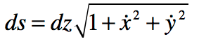
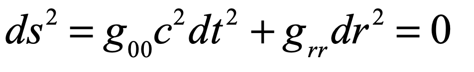
The invariant element for a light path moving radially in the Schwarzschild geometry is
The apparent speed of light is then

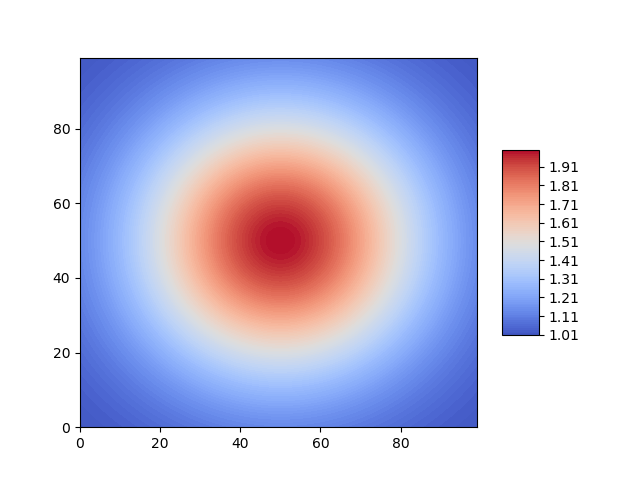
where c(r) is always less than c, when observing it from flat space. The “refractive index” of space is defined, as for any optical material, as the ratio of the constant speed divided by the observed speed

Because the Schwarzschild metric has the property
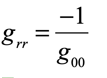
the effective refractive index of warped space-time is
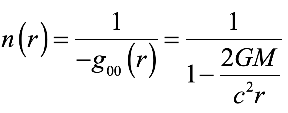
with a divergence at the Schwarzschild radius.
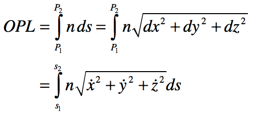
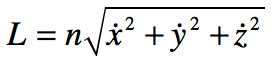
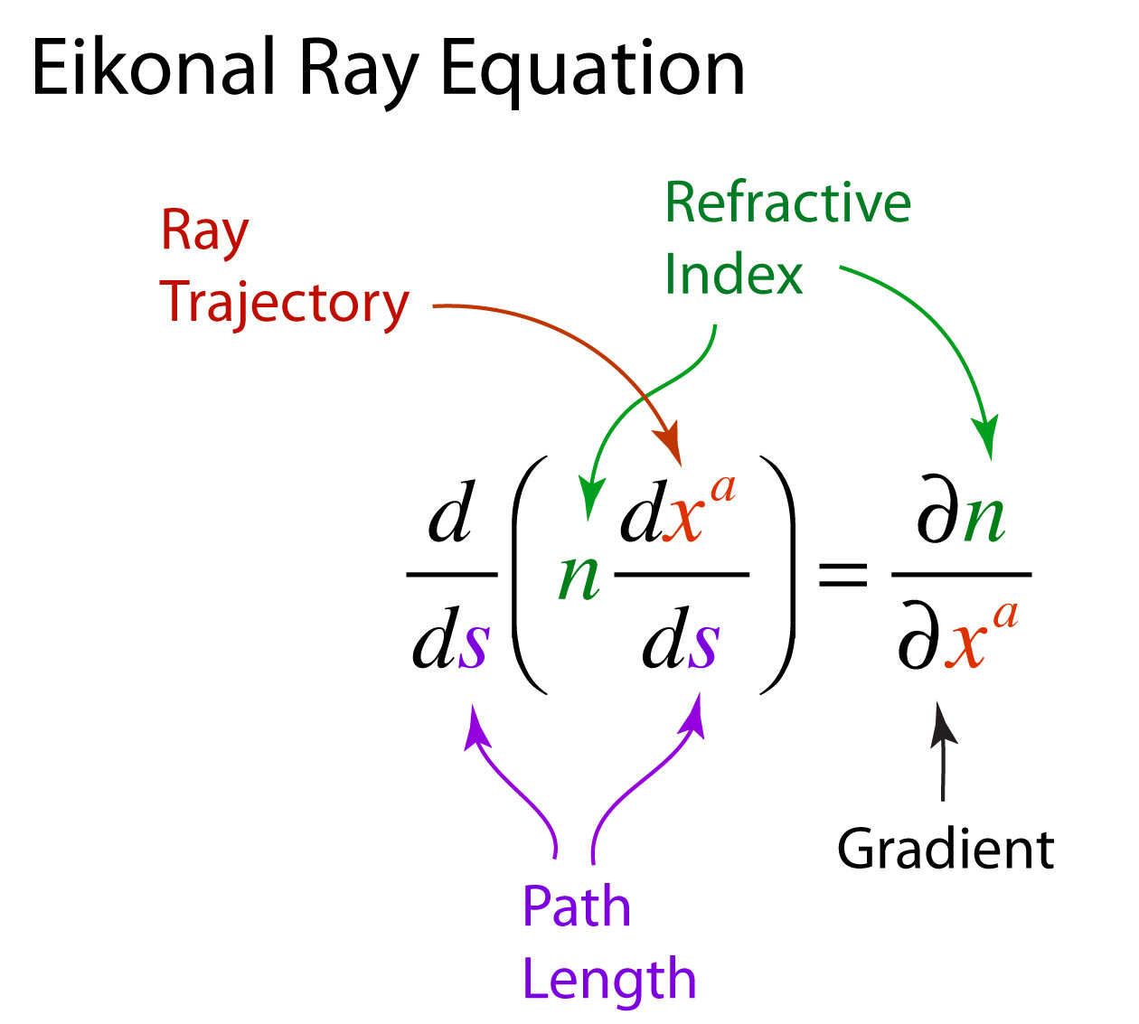
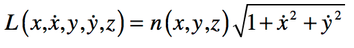
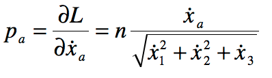
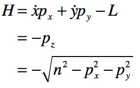
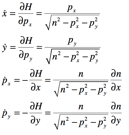
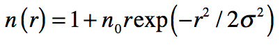
The refractive index of warped space-time in the limit of weak gravity can be used in the ray equation (also known as the Eikonal equation described in an earlier blog)
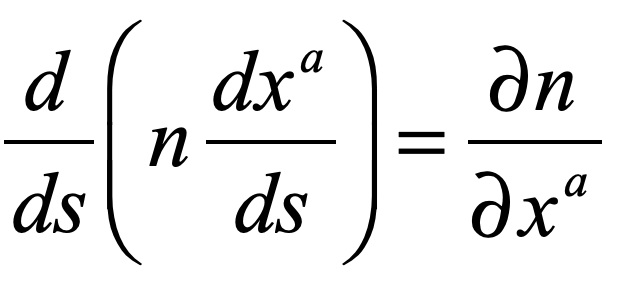
where the gradient of the refractive index of space is
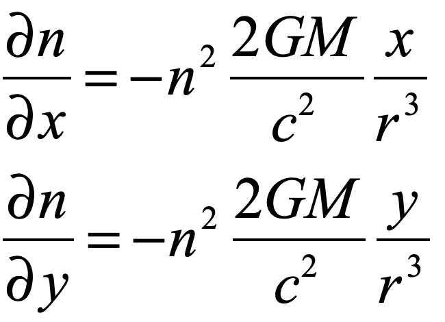
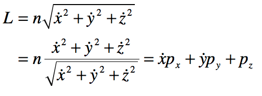
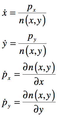
The ray equation is then a four-variable flow

These equations represent a 4-dimensional flow for a light ray confined to a plane. The trajectory of any light path is found by using an ODE solver subject to the initial conditions for the direction of the light ray. This is simple for us to do today with Python or Matlab, but it was also that could be done long before the advent of computers by early theorists of relativity like Max von Laue (1879 – 1960).
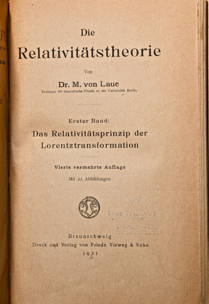
The Relativity of Max von Laue
In the Fall of 1905 in Berlin, a young German physicist by the name of Max Laue was sitting in the physics colloquium at the University listening to another Max, his doctoral supervisor Max Planck, deliver a seminar on Einstein’s new theory of relativity. Laue was struck by the simplicity of the theory, in this sense “simplistic” and hence hard to believe, but the beauty of the theory stuck with him, and he began to think through the consequences for experiments like the Fizeau experiment on partial ether drag.
Armand Hippolyte Louis Fizeau (1819 – 1896) in 1851 built one of the world’s first optical interferometers and used it to measure the speed of light inside moving fluids. At that time the speed of light was believed to be a property of the luminiferous ether, and there were several opposing theories on how light would travel inside moving matter. One theory would have the ether fully stationary, unaffected by moving matter, and hence the speed of light would be unaffected by motion. An opposite theory would have the ether fully entrained by matter and hence the speed of light in moving matter would be a simple sum of speeds. A middle theory considered that only part of the ether was dragged along with the moving matter. This was Fresnel’s partial ether drag hypothesis that he had arrived at to explain why his friend Francois Arago had not observed any contribution to stellar aberration from the motion of the Earth through the ether. When Fizeau performed his experiment, the results agreed closely with Fresnel’s drag coefficient, which seemed to settle the matter. Yet when Michelson and Morley performed their experiments of 1887, there was no evidence for partial drag.
Even after the exposition by Einstein on relativity in 1905, the disagreement of the Michelson-Morley results with Fizeau’s results was not fully reconciled until Laue showed in 1907 that the velocity addition theorem of relativity gave complete agreement with the Fizeau experiment. The velocity observed in the lab frame is found using the velocity addition theorem of special relativity. For the Fizeau experiment, water with a refractive index of n is moving with a speed v and hence the speed in the lab frame is

The difference in the speed of light between the stationary and the moving water is the difference
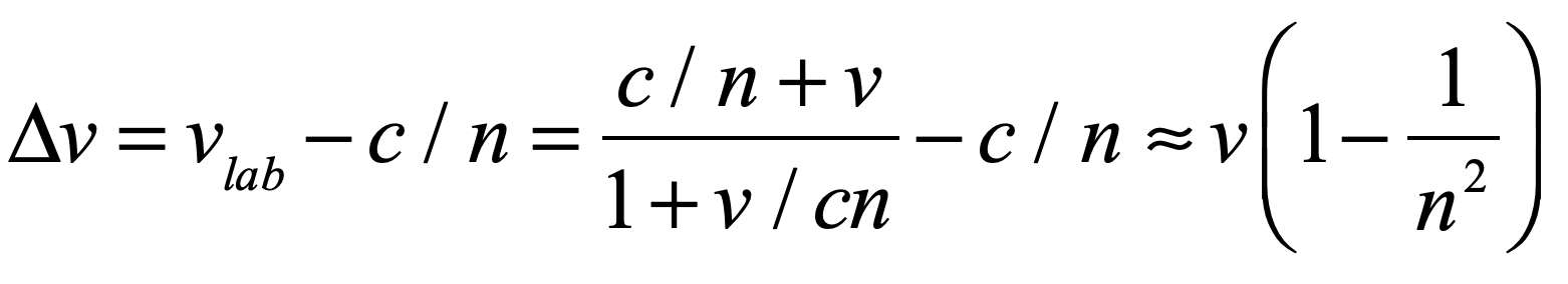
where the last term is precisely the Fresnel drag coefficient. This was one of the first definitive “proofs” of the validity of Einstein’s theory of relativity, and it made Laue one of relativity’s staunchest proponents. Spurred on by his success with the Fresnel drag coefficient explanation, Laue wrote the first monograph on relativity theory, publishing it in 1910.
A Nobel Prize for Crystal X-ray Diffraction
In 1909 Laue became a Privatdozent under Arnold Sommerfeld (1868 – 1951) at the university in Munich. In the Spring of 1912 he was walking in the Englischer Garten on the northern edge of the city talking with Paul Ewald (1888 – 1985) who was finishing his doctorate with Sommerfed studying the structure of crystals. Ewald was considering the interaction of optical wavelength with the periodic lattice when it struck Laue that x-rays would have the kind of short wavelengths that would allow the crystal to act as a diffraction grating to produce multiple diffraction orders. Within a few weeks of that discussion, two of Sommerfeld’s students (Friedrich and Knipping) used an x-ray source and photographic film to look for the predicted diffraction spots from a copper sulfate crystal. When the film was developed, it showed a constellation of dark spots for each of the diffraction orders of the x-rays scattered from the multiple periodicities of the crystal lattice. Two years later, in 1914, Laue was awarded the Nobel prize in physics for the discovery. That same year his father was elevated to the hereditary nobility in the Prussian empire and Max Laue became Max von Laue.
Von Laue was not one to take risks, and he remained conservative in many of his interests. He was immensely respected and played important roles in the administration of German science, but his scientific contributions after receiving the Nobel Prize were only modest. Yet as the Nazis came to power in the early 1930’s, he was one of the few physicists to stand up and resist the Nazi take-over of German physics. He was especially disturbed by the plight of the Jewish physicists. In 1933 he was invited to give the keynote address at the conference of the German Physical Society in Wurzburg where he spoke out against the Nazi rejection of relativity as they branded it “Jewish science”. In his speech he likened Einstein, the target of much of the propaganda, to Galileo. He said, “No matter how great the repression, the representative of science can stand erect in the triumphant certainty that is expressed in the simple phrase: And yet it moves.” Von Laue believed that truth would hold out in the face of the proscription against relativity theory by the Nazi regime. The quote “And yet it moves” is supposed to have been muttered by Galileo just after his abjuration before the Inquisition, referring to the Earth moving around the Sun. Although the quote is famous, it is believed to be a myth.
In an odd side-note of history, von Laue sent his gold Nobel prize medal to Denmark for its safe keeping with Niels Bohr so that it would not be paraded about by the Nazi regime. Yet when the Nazis invaded Denmark, to avoid having the medals fall into the hands of the Nazis, the medal was dissolved in aqua regia by a member of Bohr’s team, George de Hevesy. The gold completely dissolved into an orange liquid that was stored in a beaker high on a shelf through the war. When Denmark was finally freed, the dissolved gold was precipitated out and a new medal was struck by the Nobel committee and re-presented to von Laue in a ceremony in 1951.
The Orbits of Light Rays
Von Laue’s interests always stayed close to the properties of light and electromagnetic radiation ever since he was introduced to the field when he studied with Woldemor Voigt at Göttingen in 1899. This interest included the theory of relativity, and only a few years after Einstein published his theory of General Relativity and Gravitation, von Laue added to his earlier textbook on relativity by writing a second volume on the general theory. The new volume was published in 1920 and included the theory of the deflection of light by gravity.
One of the very few illustrations in his second volume is of light coming into interaction with a super massive gravitational field characterized by a Schwarzschild radius. (No one at the time called it a “black hole”, nor even mentioned Schwarzschild. That terminology came much later.) He shows in the drawing, how light, if incident at just the right impact parameter, would actually loop around the object. This is the first time such a diagram appeared in print, showing the trajectory of light so strongly affected by gravity.

Python Code: gravlens.py
#!/usr/bin/env python3
# -*- coding: utf-8 -*-
"""
gravlens.py
Created on Tue May 28 11:50:24 2019
@author: nolte
D. D. Nolte, Introduction to Modern Dynamics: Chaos, Networks, Space and Time, 2nd ed. (Oxford,2019)
"""

import numpy as np
import matplotlib as mpl
from mpl_toolkits.mplot3d import Axes3D
from scipy import integrate
from matplotlib import pyplot as plt
from matplotlib import cm
import time
import os

plt.close('all')

def create_circle():
	circle = plt.Circle((0,0), radius= 10, color = 'black')
	return circle

def show_shape(patch):
	ax=plt.gca()
	ax.add_patch(patch)
	plt.axis('scaled')
	plt.show()

def refindex(x,y):

    A = 10
    eps = 1e-6

    rp0 = np.sqrt(x**2 + y**2);

    n = 1/(1 - A/(rp0+eps))
    fac = np.abs((1-9*(A/rp0)**2/8))   # approx correction to Eikonal
    nx = -fac*n**2*A*x/(rp0+eps)**3
    ny = -fac*n**2*A*y/(rp0+eps)**3

    return [n,nx,ny]

def flow_deriv(x_y_z,tspan):
    x, y, z, w = x_y_z

    [n,nx,ny] = refindex(x,y)

    yp = np.zeros(shape=(4,))
    yp[0] = z/n
    yp[1] = w/n
    yp[2] = nx
    yp[3] = ny

    return yp

for loop in range(-5,30):

    xstart = -100
    ystart = -2.245 + 4*loop
    print(ystart)

    [n,nx,ny] = refindex(xstart,ystart)


    y0 = [xstart, ystart, n, 0]

    tspan = np.linspace(1,400,2000)

    y = integrate.odeint(flow_deriv, y0, tspan)

    xx = y[1:2000,0]
    yy = y[1:2000,1]


    plt.figure(1)
    lines = plt.plot(xx,yy)
    plt.setp(lines, linewidth=1)
    plt.show()
    plt.title('Photon Orbits')

c = create_circle()
show_shape(c)
axes = plt.gca()
axes.set_xlim([-100,100])
axes.set_ylim([-100,100])

# Now set up a circular photon orbit
xstart = 0
ystart = 15

[n,nx,ny] = refindex(xstart,ystart)

y0 = [xstart, ystart, n, 0]

tspan = np.linspace(1,94,1000)

y = integrate.odeint(flow_deriv, y0, tspan)

xx = y[1:1000,0]
yy = y[1:1000,1]

plt.figure(1)
lines = plt.plot(xx,yy)
plt.setp(lines, linewidth=2, color = 'black')
plt.show()
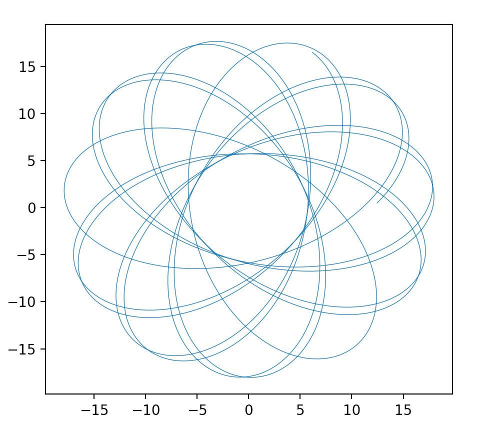
One of the most striking effects of gravity on photon trajectories is the possibility for a photon to orbit a black hole in a circular orbit. This is shown in Fig. 3 as the black circular ring for a photon at a radius equal to 1.5 times the Schwarzschild radius. This radius defines what is known as the photon sphere. However, the orbit is not stable. Slight deviations will send the photon spiraling outward or inward.
The Eikonal approximation does not strictly hold under strong gravity, but the Eikonal equations with the effective refractive index of space still yield semi-quantitative behavior. In the Python code, a correction factor is used to match the theory to the circular photon orbits, while still agreeing with trajectories far from the black hole. The results of the calculation are shown in Fig. 3. For large impact parameters, the rays are deflected through a finite angle. At a critical impact parameter, near 3 times the Schwarzschild radius, the ray loops around the black hole. For smaller impact parameters, the rays are captured by the black hole.

Photons pile up around the black hole at the photon sphere. The first image ever of the photon sphere of a black hole was made earlier this year (announced April 10, 2019). The image shows the shadow of the supermassive black hole in the center of Messier 87 (M87), an elliptical galaxy 55 million light-years from Earth. This black hole is 6.5 billion times the mass of the Sun. Imaging the photosphere required eight ground-based radio telescopes placed around the globe, operating together to form a single telescope with an optical aperture the size of our planet. The resolution of such a large telescope would allow one to image a half-dollar coin on the surface of the Moon, although this telescope operates in the radio frequency range rather than the optical.

By David D. Nolte, July 29, 2019
Further Reading
B. Lavenda, The Optical Properties of Gravity, J. Mod. Phys, 8 8-3-838 (2017)