Posts by David D. Nolte

David D. Nolte is the Edward M. Purcell Distinguished Professor of Physics and Astronomy at Purdue University. He research has pioneered the physics and applications of dynamic holography, the BioCD, and dynamic contrast optical coherence tomography (DC-OCT). He received his baccalaureate from Cornell University, his PhD from the University of California at Berkeley, and had a post-doctoral appointment at AT&T Bell Labs before joining the faculty at Purdue. He is a Fellow of the Optical Society of America, a Fellow of the American Physical Society and a Fellow of the AAAS. He received the Herbert Newby McCoy Award of Purdue University and is the technical founder of two biotech startup companies in diagnostic screening and analysis. He has written several popular science books, including Interference (Oxford, 2023), Galileo Unbound (Oxford, 2018), and Mind at Light Speed (Free Press, 2001).

September 15, 2019October 24, 2023 by David D. Nolte

Karl Schwarzschild’s Radius: How Fame Eclipsed a Physicist’s own Legacy

In an ironic twist of the history of physics, Karl Schwarzschild’s fame has eclipsed his own legacy. When asked who was Karl Schwarzschild (1873 – 1916), you would probably say he’s the guy who solved Einstein’s Field Equations of General Relativity and discovered the radius of black holes. You may also know that he accomplished this Herculean feat while dying slowly behind the German lines on the Eastern Front in WWI. But asked what else he did, and you would probably come up blank. Yet Schwarzschild was one of the most wide-ranging physicists at the turn of the 20^th century, which is saying something, because it places him into the same pantheon as Planck, Lorentz, Poincaré and Einstein. Let’s take a look at the part of his career that hides in the shadow of his own radius.

A Radius of Interest

Karl Schwarzschild was born in Frankfurt, Germany, shortly after the Franco-Prussian war thrust Prussia onto the world stage as a major political force in Europe. His family were Jewish merchants of longstanding reputation in the city, and Schwarzschild’s childhood was spent in the vibrant Jewish community. One of his father’s friends was a professor at a university in Frankfurt, whose son, Paul Epstein (1871 – 1939), became a close friend of Karl’s at the Gymnasium. Schwarzshild and Epstein would partially shadow each other’s careers despite the fact that Schwarzschild became an astronomer while Epstein became a famous mathematician and number theorist. This was in part because Schwarzschild had large radius of interests that spanned the breadth of current mathematics and science, practicing both experiments and theory.

Schwarzschild’s application of the Hamiltonian formalism for quantum systems set the stage for the later adoption of Hamiltonian methods in quantum mechanics. He came dangerously close to stating the uncertainty principle that catapulted Heisenberg to fame.

By the time Schwarzschild was sixteen, he had taught himself the mathematics of celestial mechanics to such depth that he published two papers on the orbits of binary stars. He also became fascinated in astronomy and purchased lenses and other materials to construct his own telescope. His interests were helped along by Epstein, two years older and whose father had his own private observatory. When Epstein went to study at the University of Strasbourg (then part of the German Federation) Schwarzschild followed him. But Schwarzschild’s main interest in astronomy diverged from Epstein’s main interest in mathematics, and Schwarzschild transferred to the University of Munich where he studied under Hugo von Seeliger (1849 – 1924), the premier German astronomer of his day. Epstein remained at Strasbourg where he studied under Bruno Christoffel (1829 – 1900) and eventually became a professor, but he was forced to relinquish the post when Strasbourg was ceded to France after WWI.

The Birth of Stellar Interferometry

Until the Hubble space telescope was launched in 1990 no star had ever been resolved as a direct image. Within a year of its launch, using its spectacular resolving power, the Hubble optics resolved—just barely—the red supergiant Betelgeuse. No other star (other than the Sun) is close enough or big enough to image the stellar disk, even for the Hubble far above our atmosphere. The reason is that the diameter of the optical lenses and mirrors of the Hubble—as big as they are at 2.4 meter diameter—still produce a diffraction pattern that smears the image so that stars cannot be resolved. Yet information on the size of a distant object is encoded as phase in the light waves that are emitted from the object, and this phase information is accessible to interferometry.

The first physicist who truly grasped the power of optical interferometry and who understood how to design the first interferometric metrology systems was the French physicist Armand Hippolyte Louis Fizeau (1819 – 1896). Fizeau became interested in the properties of light when he collaborated with his friend Léon Foucault (1819–1868) on early uses of photography. The two then embarked on a measurement of the speed of light but had a falling out before the experiment could be finished, and both continued the pursuit independently. Fizeau achieved the first measurement using a toothed wheel rotating rapidly [1], while Foucault came in second using a more versatile system with a spinning mirror [2]. Yet Fizeau surpassed Foucault in optical design and became an expert in interference effects. Interference apparatus had been developed earlier by Augustin Fresnel (the Fresnel bi-prism 1819), Humphrey Lloyd (Lloyd’s mirror 1834) and Jules Jamin (Jamin’s interferential refractor 1856). They had found ways of redirecting light using refraction and reflection to cause interference fringes. But Fizeau was one of the first to recognize that each emitting region of a light source was coherent with itself, and he used this insight and the use of lenses to design the first interferometer.

Fizeau’s interferometer used a lens with a with a tight focal spot masked off by an opaque screen with two open slits. When the masked lens device was focused on an intense light source it produced two parallel pencils of light that were mutually coherent but spatially separated. Fizeau used this apparatus to measure the speed of light in moving water in 1859 [3].

Fig. 1 Optical configuration of the source element of the Fizeau refractometer.

The working principle of the Fizeau refractometer is shown in Fig. 1. The light source is at the bottom, and it is reflected by the partially-silvered beam splitter to pass through the lens and the mask containing two slits. (Only the light paths that pass through the double-slit mask on the lens are shown in the figure.) The slits produce two pencils of mutually coherent light that pass through a system (in the famous Fizeau ether drag experiment it was along two tubes of moving water) and are returned through the same slits, and they intersect at the view port where they produce interference fringes. The fringe spacing is set by the separation of the two slits in the mask. The Rayleigh region of the lens defines a region of spatial coherence even for a so-called “incoherent” source. Therefore, this apparatus, by use of the lens, could convert an incoherent light source into a coherent probe to test the refractive index of test materials, which is why it was called a refractometer.

Fizeau became adept at thinking of alternative optical designs of his refractometer and alternative applications. In an address to the French Physical Society in 1868 he suggested that the double-slit mask could be used on a telescope to determine sizes of distant astronomical objects [4]. There were several subsequent attempts to use Fizeau’s configuration in astronomical observations, but none were conclusive and hence were not widely known.

An optical configuration and astronomical application that was very similar to Fizeau’s idea was proposed by Albert Michelson in 1890 [5]. He built the apparatus and used it to successfully measure the size of several moons of Jupiter [6]. The configuration of the Michelson stellar interferometer is shown in Fig. 2. Light from a distant star passes through two slits in the mask in front of the collecting optics of a telescope. When the two pencils of light intersect at the view port, they produce interference fringes. Because of the finite size of the stellar source, the fringes are partially washed out. By adjusting the slit separation, a certain separation can be found where the fringes completely wash out. The size of the star is then related to the separation of the slits for which the fringe visibility vanishes. This simple principle allows this type of stellar interferometry to measure the size of stars that are large and relatively close to Earth. However, if stars are too far away even this approach cannot be used to measure their sizes because telescopes aren’t big enough. This limitation is currently being bypassed by the use of long-baseline optical interferometers.

Fig. 2 Optical configuration of the Michelson stellar interferometer. Fringes at the view port are partially washed out by the finite size of the star. By adjusting the slit separation, the fringes can be made to vanish entirely, yielding an equation that can be solved for the size of the star.

One of the open questions in the history of interferometry is whether Michelson was aware of Fizeau’s proposal for the stellar interferometer made in 1868. Michelson was well aware of Fizeau’s published research and acknowledged him as a direct inspiration of his own work in interference effects. But Michelson also was unaware of the undercurrents in the French school of optical interference. When he visited Paris in 1881, he met with many of the leading figures in this school (including Lippmann and Cornu), but there is no mention or any evidence that he met with Fizeau. By this time Fizeau’s wife had passed away, and Fizeau spent most of his time in seclusion at his home outside Paris. Therefore, it is unlikely that he would have been present during Michelson’s visit. Because Michelson viewed Fizeau with such awe and respect, if he had met him, he most certainly would have mentioned it. Therefore, Michelson’s invention of the stellar interferometer can be considered with some confidence to be a case of independent discovery. It is perhaps not surprising that he hit on the same idea that Fizeau had in 1868, because Michelson was one of the few physicists who understood coherence and interference at the same depth as Fizeau.

Schwarzschild’s Stellar Interferometer

The physics of the Michelson stellar interferometer is very similar to the physics of Young’s double slit experiment. The two slits in the aperture mask of the telescope objective act to produce a simple sinusoidal interference pattern at the image plane of the optical system. The size of the stellar diameter is determined by using the wash-out effect of the fringes caused by the finite stellar size. However, it is well known to physicists who work with diffraction gratings that a multiple-slit interference pattern has a much greater resolving power than a simple double slit.

This realization must have hit von Seeliger and Schwarzschild, working together at Munich, when they saw the publication of Michelson’s theoretical analysis of his stellar interferometer in 1890, followed by his use of the apparatus to measure the size of Jupiter’s moons. Schwarzschild and von Seeliger realized that by replacing the double-slit mask with a multiple-slit mask, the widths of the interference maxima would be much narrower. Such a diffraction mask on a telescope would cause a star to produce a multiple set of images on the image plane of the telescope associated with the multiple diffraction orders. More interestingly, if the target were a binary star, the diffraction would produce two sets of diffraction maxima—a double image! If the “finesse” of the grating is high enough, the binary star separation could be resolved as a doublet in the diffraction pattern at the image, and the separation could be measured, giving the angular separation of the two stars of the binary system. Such an approach to the binary separation would be a direct measurement, which was a distinct and clever improvement over the indirect Michelson configuration that required finding the extinction of the fringe visibility.

Schwarzschild enlisted the help of a fine German instrument maker to create a multiple slit system that had an adjustable slit separation. The device is shown in Fig. 3 from Schwarzschild’s 1896 publication on the use of the stellar interferometer to measure the separation of binary stars [7]. The device is ingenious. By rotating the chain around the gear on the right-hand side of the apparatus, the two metal plates with four slits could be raised or lowered, cause the projection onto the objective plane to have variable slit spacings. In the operation of the telescope, the changing height of the slits does not matter, because they are near a conjugate optical plane (the entrance pupil) of the optical system. Using this adjustable multiple slit system, Schwarzschild (and two colleagues he enlisted) made multiple observations of well-known binary star systems, and they calculated the star separations. Several of their published results are shown in Fig. 4.

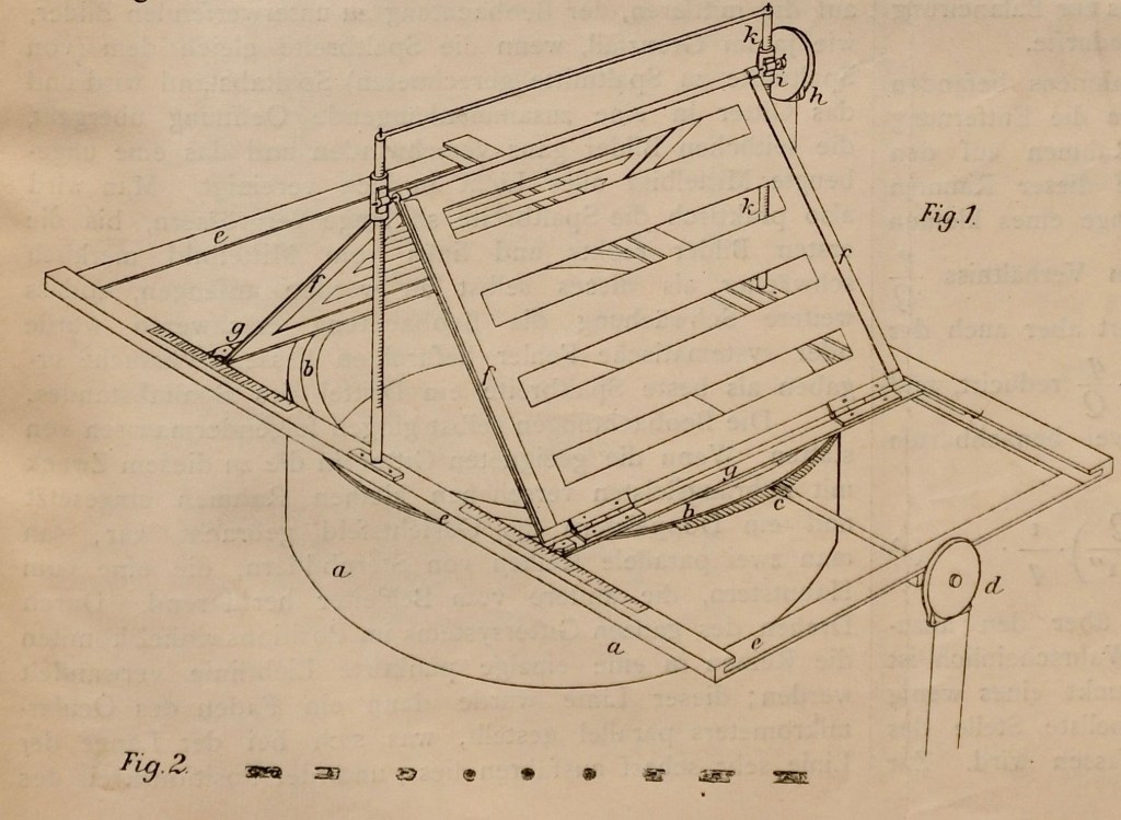
Fig. 3 Illustration from Schwarzschild’s 1896 paper describing an improvement of the Michelson interferometer for measuring the separation of binary star systems Ref. [7].

Fig. 4 Data page from Schwarzschild’s 1896 paper measuring the angular separation of two well-known binary star systems: gamma Leonis and chsi Ursa Major. Ref. [7]

Schwarzschild’s publication demonstrated one of the very first uses of stellar interferometry—well before Michelson himself used his own configuration to measure the diameter of Betelgeuse in 1920. Schwarzschild’s major achievement was performed before he had received his doctorate, on a topic orthogonal to his dissertation topic. Yet this fact is virtually unknown to the broader physics community outside of astronomy. If he had not become so famous later for his solution of Einstein’s field equations, Schwarzschild nonetheless might have been famous for his early contributions to stellar interferometry. But even this was not the end of his unique contributions to physics.

Adiabatic Physics

As Schwarzschild worked for his doctorate under von Seeliger, his dissertation topic was on new theories by Henri Poincaré (1854 – 1912) on celestial mechanics. Poincaré had made a big splash on the international stage with the publication of his prize-winning memoire in 1890 on the three-body problem. This is the publication where Poincaré first described what would later become known as chaos theory. The memoire was followed by his volumes on “New Methods in Celestial Mechanics” published between 1892 and 1899. Poincaré’s work on celestial mechanics was based on his earlier work on the theory of dynamical systems where he discovered important invariant theorems, such as Liouville’s theorem on the conservation of phase space volume. Schwarzshild applied Poincaré’s theorems to problems in celestial orbits. He took his doctorate in 1896 and received a post at an astronomical observatory outside Vienna.

While at Vienna, Schwarzschild performed his most important sustained contributions to the science of astronomy. Astronomical observations had been dominated for centuries by the human eye, but photographic techniques had been making steady inroads since the time of Hermann Carl Vogel (1841 – 1907) in the 1880’s at the Potsdam observatory. Photographic plates were used primarily to record star positions but were known to be unreliable for recording stellar intensities. Schwarzschild developed a “out-of-focus” technique that blurred the star’s image, while making it larger and easier to measure the density of the exposed and developed photographic emulsions. In this way, Schwarzschild measured the magnitudes of 367 stars. Two of these stars had variable magnitudes that he was able to record and track. Schwarzschild correctly explained the intensity variation caused by steady oscillations in heating and cooling of the stellar atmosphere. This work established the properties of these Cepheid variables which would become some of the most important “standard candles” for the measurement of cosmological distances. Based on the importance of this work, Schwarzschild returned to Munich as a teacher in 1899 and subsequently was appointed in 1901 as the director of the observatory at Göttingen established by Gauss eighty years earlier.

Schwarzschild’s years at Göttingen brought him into contact with some of the greatest mathematicians and physicists of that era. The mathematicians included Felix Klein, David Hilbert and Hermann Minkowski. The physicists included von Laue, a student of Woldemar Voigt. This period was one of several “golden ages” of Göttingen. The first golden age was the time of Gauss and Riemann in the mid-1800’s. The second golden age, when Schwarzschild was present, began when Felix Klein arrived at Göttingen and attracted the top mathematicians of the time. The third golden age of Göttingen was the time of Born and Jordan and Heisenberg at the birth of quantum mechanics in the mid 1920’s.

In 1906, the Austrian Physicist Paul Ehrenfest, freshly out of his PhD under the supervision of Boltzmann, arrived at Göttingen only weeks before Boltzmann took his own life. Felix Klein at Göttingen had been relying on Boltzmann to provide a comprehensive review of statistical mechanics for the Mathematical Encyclopedia, so he now entrusted this project to the young Ehrenfest. It was a monumental task, which was to take him and his physicist wife Tatyanya nearly five years to complete. Part of the delay was the desire by the Ehrenfests to close some open problems that remained in Boltzmann’s work. One of these was a mechanical theorem of Boltzmann’s that identified properties of statistical mechanical systems that remained unaltered through a very slow change in system parameters. These properties would later be called adiabatic invariants by Einstein.

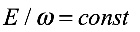
Ehrenfest recognized that Wien’s displacement law, which had been a guiding light for Planck and his theory of black body radiation, had originally been derived by Wien using classical principles related to slow changes in the volume of a cavity. Ehrenfest was struck by the fact that such slow changes would not induce changes in the quantum numbers of the quantized states, and hence that the quantum numbers must be adiabatic invariants of the black body system. This not only explained why Wien’s displacement law continued to hold under quantum as well as classical considerations, but it also explained why Planck’s quantization of the energy of his simple oscillators was the only possible choice. For a classical harmonic oscillator, the ratio of the energy of oscillation to the frequency of oscillation is an adiabatic invariant, which is immediately recognized as Planck’s quantum condition .

Ehrenfest published his observations in 1913 [8], the same year that Bohr published his theory of the hydrogen atom, so Ehrenfest immediately applied the theory of adiabatic invariants to Bohr’s model and discovered that the quantum condition for the quantized energy levels was again the adiabatic invariants of the electron orbits, and not merely a consequence of integer multiples of angular momentum, which had seemed somewhat ad hoc.

After eight exciting years at Göttingen, Schwarzschild was offered the position at the Potsdam Observatory in 1909 upon the retirement from that post of the famous German astronomer Carl Vogel who had made the first confirmed measurements of the optical Doppler effect. Schwarzschild accepted and moved to Potsdam with a new family. His son Martin Schwarzschild would follow him into his profession, becoming a famous astronomer at Princeton University and a theorist on stellar structure. At the outbreak of WWI, Schwarzschild joined the German army out of a sense of patriotism. Because of his advanced education he was made an officer of artillery with the job to calculate artillery trajectories, and after a short time on the Western Front in Belgium was transferred to the Eastern Front in Russia. Though he was not in the trenches, he was in the midst of the chaos to the rear of the front. Despite this situation, he found time to pursue his science through the year 1915.

Schwarzschild was intrigued by Ehrenfest’s paper on adiabatic invariants and their similarity to several of the invariant theorems of Poincaré that he had studied for his doctorate. Up until this time, mechanics had been mostly pursued through the Lagrangian formalism which could easily handle generalized forces associated with dissipation. But celestial mechanics are conservative systems for which the Hamiltonian formalism is a more natural approach. In particular, the Hamilton-Jacobi canonical transformations made it particularly easy to find pairs of generalized coordinates that had simple periodic behavior. In his published paper [9], Schwarzschild called these “Action-Angle” coordinates because one was the action integral that was well-known in the principle of “Least Action”, and the other was like an angle variable that changed steadily in time (see Fig. 5). Action-angle coordinates have come to form the foundation of many of the properties of Hamiltonian chaos, Hamiltonian maps, and Hamiltonian tapestries.

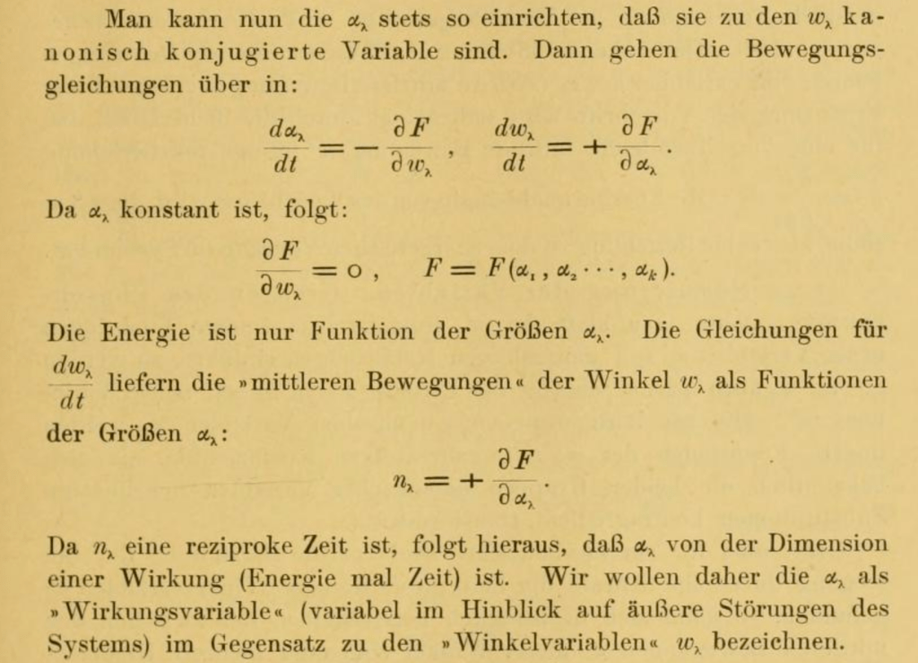
Fig. 5 Description of the canonical transformation to action-angle coordinates (Ref. [9] pg. 549). Schwarzschild names the new coordinates “Wirkungsvariable” and “Winkelvariable”.

During lulls in bombardments, Schwarzschild translated the Hamilton-Jacobi methods of celestial mechanics to apply them to the new quantum mechanics of the Bohr orbits. The phrase “quantum mechanics” had not yet been coined (that would come ten years later in a paper by Max Born), but it was clear that the Bohr quantization conditions were a new type of mechanics. The periodicities that were inherent in the quantum systems were natural properties that could be mapped onto the periodicities of the angle variables, while Ehrenfest’s adiabatic invariants could be mapped onto the slowly varying action integrals. Schwarzschild showed that action-angle coordinates were the only allowed choice of coordinates, because they enabled the separation of the Hamilton-Jacobi equations and hence provided the correct quantization conditions for the Bohr electron orbits. Later, when Sommerfeld published his quantized elliptical orbits in 1916, the multiplicity of quantum conditions and orbits had caused concern, but Ehrenfest came to the rescue, showing that each of Sommerfeld’s quantum conditions were precisely Schwarzschild’s action-integral invariants of the classical electron dynamics [10].

The works by Schwarzschild, and a closely-related paper that amplified his ideas published by his friend Paul Epstein several months later [11], were the first to show the power of the Hamiltonian formulation of dynamics for quantum systems, foreshadowing the future importance of Hamiltonians for quantum theory. An essential part of the Hamiltonian formalism is the concept of phase space. In his paper, Schwarzschild showed that the phase space of quantum systems was divided into small but finite elementary regions whose areas were equal to Planck’s constant h-bar (see Fig. 6). The areas were products of a small change in momentum coordinate Delta-p and a corresponding small change in position coordinate Delta-x. Therefore, the product DxDp = h-bar. This observation, made in 1915 by Schwarzschild, was only one step away from Heisenberg’s uncertainty relation, twelve years before Heisenberg discovered it. However, in 1915 Born’s probabilistic interpretation of quantum mechanics had not yet been made, nor the idea of measurement uncertainty, so Schwarzschild did not have the appropriate context in which to have made the leap to the uncertainty principle. However, by introducing the action-angle coordinates as well as the Hamiltonian formalism applied to quantum systems, with the natural structure of phase space, Schwarzschild laid the foundation for the future developments in quantum theory made by the next generation.

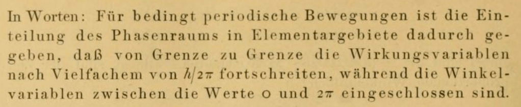
Fig. 6 Expression of the division of phase space into elemental areas of action equal to h-bar (Ref. [9] pg. 550).

All Quiet on the Eastern Front

Towards the end of his second stay in Munich in 1900, prior to joining the Göttingen faculty, Schwarzschild had presented a paper at a meeting of the German Astronomical Society held in Heidelberg in August. The topic was unlike anything he had tackled before. It considered the highly theoretical question of whether the universe was non-Euclidean, and more specifically if it had curvature. He concluded from observation that if the universe were curved, the radius of curvature must be larger than between 50 light years and 2000 light years, depending on whether the geometry was hyperbolic or elliptical. Schwarzschild was working out ideas of differential geometry and applying them to the universe at large at a time when Einstein was just graduating from the ETH where he skipped his math classes and had his friend Marcel Grossmann take notes for him.

The topic of Schwarzschild’s talk tells an important story about the warping of historical perspective by the “great man” syndrome. In this case the great man is Einstein who is today given all the credit for discovering the warping of space. His development of General Relativity is often portrayed as by a lone genius in the wilderness performing a blazing act of creation out of the void. In fact, non-Euclidean geometry had been around for some time by 1900—five years before Einstein’s Special Theory and ten years before his first publications on the General Theory. Gauss had developed the idea of intrinsic curvature of a manifold fifty years earlier, amplified by Riemann. By the turn of the century alternative geometries were all the rage, and Schwarzschild considered whether there were sufficient astronomical observations to set limits on the size of curvature of the universe. But revisionist history is just as prevalent in physics as in any field, and when someone like Einstein becomes so big in the mind’s eye, his shadow makes it difficult to see all the people standing behind him.

This is not meant to take away from the feat that Einstein accomplished. The General Theory of Relativity, published by Einstein in its full form in 1915 was spectacular [12]. Einstein had taken vague notions about curved spaces and had made them specific, mathematically rigorous and intimately connected with physics through the mass-energy source term in his field equations. His mathematics had gone beyond even what his mathematician friend and former collaborator Grossmann could achieve. Yet Einstein’s field equations were nonlinear tensor differential equations in which the warping of space depended on the strength of energy fields, but the configuration of those energy fields depended on the warping of space. This type of nonlinear equation is difficult to solve in general terms, and Einstein was not immediately aware of how to find the solutions to his own equations.

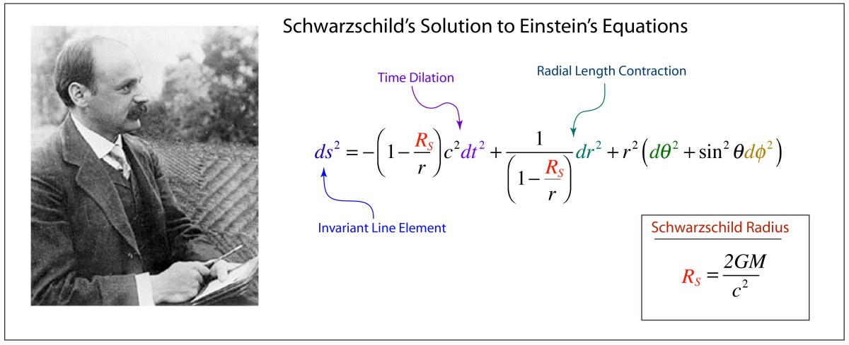
Therefore, it was no small surprise to him when he received a letter from the Eastern Front from an astronomer he barely knew who had found a solution—a simple solution (see Fig. 7) —to his field equations. Einstein probably wondered how he could have missed it, but he was generous and forwarded the letter to the Reports of the Prussian Physical Society where it was published in 1916 [13].

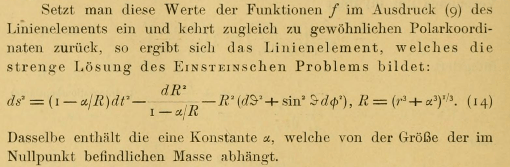
Fig. 7 Schwarzschild’s solution of the Einstein Field Equations (Ref. [13] pg. 194).

In the same paper, Schwarzschild used his exact solution to find the exact equation that described the precession of the perihelion of Mercury that Einstein had only calculated approximately. The dynamical equations for Mercury are shown in Fig. 8.

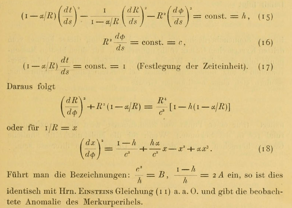
Fig. 8 Explanation for the precession of the perihelion of Mercury ( Ref. [13] pg. 195)

Schwarzschild’s solution to Einstein’s Field Equation of General Relativity was not a general solution, even for a point mass. He had constants of integration that could have arbitrary values, such as the characteristic length scale that Schwarzschild called “alpha”. It was David Hilbert who later expanded upon Schwarzschild’s work, giving the general solution and naming the characteristic length scale (where the metric diverges) after Schwarzschild. This is where the phrase “Schwarzschild Radius” got its name, and it stuck. In fact it stuck so well that Schwarzschild’s radius has now eclipsed much of the rest of Schwarzschild’s considerable accomplishments.

Unfortunately, Schwarzschild’s accomplishments were cut short when he contracted an autoimmune disease that may have been hereditary. It is ironic that in the carnage of the Eastern Front, it was a genetic disease that caused his death at the age of 42. He was already suffering from the effects of the disease as he worked on his last publications. He was sent home from the front to his family in Potsdam where he passed away several months later having shepherded his final two papers through the publication process. His last paper, on the action-angle variables in quantum systems , was published on the day that he died.

Schwarzschild’s Legacy

Schwarzschild’s legacy was assured when he solved Einstein’s field equations and Einstein communicated it to the world. But his hidden legacy is no less important.

Schwarzschild’s application of the Hamiltonian formalism of canonical transformations and phase space for quantum systems set the stage for the later adoption of Hamiltonian methods in quantum mechanics. He came dangerously close to stating the uncertainty principle that catapulted Heisenberg to later fame, although he could not express it in probabilistic terms because he came too early.

Schwarzschild is considered to be the greatest German astronomer of the last hundred years. This is in part based on his work at the birth of stellar interferometry and in part on his development of stellar photometry and the calibration of the Cepheid variable stars that went on to revolutionize our view of our place in the universe. Solving Einsteins field equations was just a sideline for him, a hobby to occupy his active and curious mind.

The Physics of Life, the Universe and Everyting:

References

[1] Fizeau, H. L. (1849). “Sur une expérience relative à la vitesse de propagation de la lumière.” Comptes rendus de l’Académie des sciences 29: 90–92, 132.

[2] Foucault, J. L. (1862). “Détermination expérimentale de la vitesse de la lumière: parallaxe du Soleil.” Comptes rendus de l’Académie des sciences 55: 501–503, 792–596.

[3] Fizeau, H. (1859). “Sur les hypothèses relatives à l’éther lumineux.” Ann. Chim. Phys. Ser. 4 57: 385–404.

[4] Fizeau, H. (1868). “Prix Bordin: Rapport sur le concours de l’annee 1867.” C. R. Acad. Sci. 66: 932.

[5] Michelson, A. A. (1890). “I. On the application of interference methods to astronomical measurements.” The London, Edinburgh, and Dublin Philosophical Magazine and Journal of Science 30(182): 1-21.

[6] Michelson, A. A. (1891). “Measurement of Jupiter’s Satellites by Interference.” Nature 45(1155): 160-161.

[7] Schwarzschild, K. (1896). “Über messung von doppelsternen durch interferenzen.” Astron. Nachr. 3335: 139.

[8] P. Ehrenfest, “Een mechanische theorema van Boltzmann en zijne betrekking tot de quanta theorie (A mechanical theorem of Boltzmann and its relation to the theory of energy quanta),” Verslag van de Gewoge Vergaderingen der Wis-en Natuurkungige Afdeeling, vol. 22, pp. 586-593, 1913.

[9] Schwarzschild, K. (1916). “Quantum hypothesis.” Sitzungsberichte Der Koniglich Preussischen Akademie Der Wissenschaften: 548-568.

[10] P. Ehrenfest, “Adiabatic invariables and quantum theory,” Annalen Der Physik, vol. 51, pp. 327-352, Oct 1916.

[11] Epstein, P. S. (1916). “The quantum theory.” Annalen Der Physik 51(18): 168-188.

[12] Einstein, A. (1915). “On the general theory of relativity.” Sitzungsberichte Der Koniglich Preussischen Akademie Der Wissenschaften: 778-786.

[13] Schwarzschild, K. (1916). “Über das Gravitationsfeld eines Massenpunktes nach der Einstein’schen Theorie.” Sitzungsberichte der Königlich-Preussischen Akademie der Wissenschaften: 189.

August 26, 2019June 1, 2023 by David D. Nolte

Limit-Cycle Oscillators: The Fast and the Slow of Grandfather Clocks

Imagine in your mind the stately grandfather clock. The long slow pendulum swinging back and forth so purposefully with such majesty. It harks back to slower simpler times—seemingly Victorian in character, although their origins go back to Christiaan Huygens in 1656. In introductory physics classes the dynamics of the pendulum is taught as one of the simplest simple harmonic oscillators, only a bit more complicated than a mass on a spring.

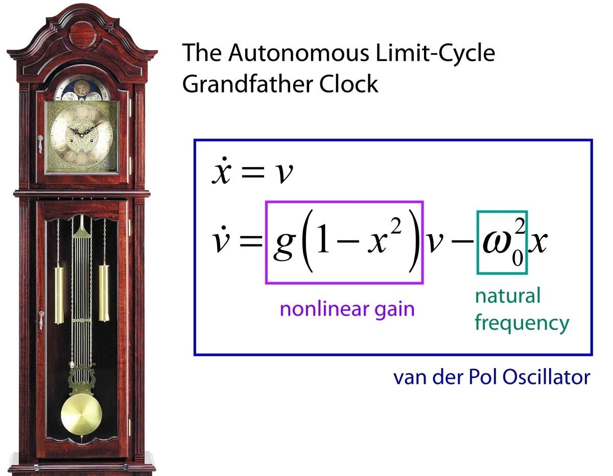
But don’t be fooled! This simplicity is an allusion, for the pendulum clock lies at the heart of modern dynamics. It is a nonlinear autonomous oscillator with system gain that balances dissipation to maintain a dynamic equilibrium that ticks on resolutely as long as some energy source can continue to supply it (like the heavy clock weights).

This analysis has converted the two-dimensional dynamics of the autonomous oscillator to a simple one-dimensional dynamics with a stable fixed point.

The dynamic equilibrium of the grandfather clock is known as a limit cycle, and they are the central feature of autonomous oscillators. Autonomous oscillators are one of the building blocks of complex systems, providing the fundamental elements for biological oscillators, neural networks, business cycles, population dynamics, viral epidemics, and even the rings of Saturn. The most famous autonomous oscillator (after the pendulum clock) is named for a Dutch physicist, Balthasar van der Pol (1889 – 1959), who discovered the laws that govern how electrons oscillate in vacuum tubes. But this highly specialized physics problem has expanded to become the new guiding paradigm for the fundamental oscillating element of modern dynamics—the van der Pol oscillator.

The van der Pol Oscillator

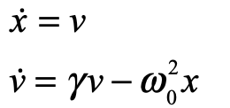
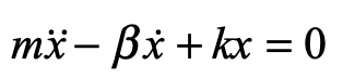
The van der Pol (vdP) oscillator begins as a simple harmonic oscillator (SHO) in which the dissipation (loss of energy) is flipped to become gain of energy. This is as simple as flipping the sign of the damping term in the SHO

where β is positive. This 2^nd-order ODE is re-written into a dynamical flow as

where γ = β/m is the system gain. Clearly, the dynamics of this SHO with gain would lead to run-away as the oscillator grows without bound.

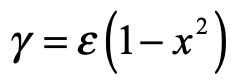
But no real-world system can grow indefinitely. It has to eventually be limited by things such as inelasticity. One of the simplest ways to include such a limiting process in the mathematical model is to make the gain get smaller at larger amplitudes. This can be accomplished by making the gain a function of the amplitude x as

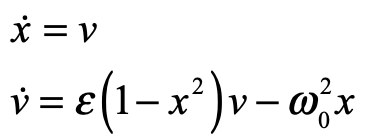
When the amplitude x gets large, the gain decreases, becoming zero and changing sign when x = 1. Putting this amplitude-dependent gain into the SHO equation yields

This is the van der Pol equation. It is the quintessential example of a nonlinear autonomous oscillator.

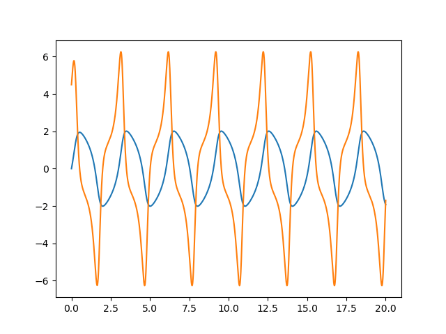
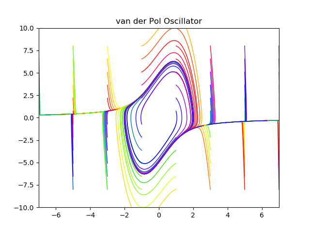
When the parameter ε is large, the vdP oscillator has can behave in strongly nonlinear ways, with strongly nonlinear and nonharmonic oscillations. An example is shown in Fig. 2 for a = 5 and b = 2.5. The oscillation is clearly non-harmonic.

Fig. 1 Time trace of the position and velocity of the vdP oscillator with w0 = 5 and ε = 2.5.

Fig. 2 State-space portrait of the vdP flow lines for w0 = 5 and ε = 2.5.

#!/usr/bin/env python3
# -*- coding: utf-8 -*-
"""
Created on Mon Apr 16 07:38:57 2018
@author: David Nolte
D. D. Nolte, Introduction to Modern Dynamics: Chaos, Networks, Space and Time, 2nd ed. (Oxford,2019)
"""
import numpy as np
from scipy import integrate
from matplotlib import pyplot as plt

plt.close('all')

def solve_flow(param,lim = [-3,3,-3,3],max_time=10.0):
# van der pol 2D flow 
    def flow_deriv(x_y, t0, alpha,beta):
        x, y = x_y
        return [y,-alpha*x+beta*(1-x**2)*y]
    
    plt.figure()
    xmin = lim[0]
    xmax = lim[1]
    ymin = lim[2]
    ymax = lim[3]
    plt.axis([xmin, xmax, ymin, ymax])

    N=144
    colors = plt.cm.prism(np.linspace(0, 1, N))
    
    x0 = np.zeros(shape=(N,2))
    ind = -1
    for i in range(0,12):
        for j in range(0,12):
            ind = ind + 1;
            x0[ind,0] = ymin-1 + (ymax-ymin+2)*i/11
            x0[ind,1] = xmin-1 + (xmax-xmin+2)*j/11
             
    # Solve for the trajectories
    t = np.linspace(0, max_time, int(250*max_time))
    x_t = np.asarray([integrate.odeint(flow_deriv, x0i, t, param)
                      for x0i in x0])

    for i in range(N):
        x, y = x_t[i,:,:].T
        lines = plt.plot(x, y, '-', c=colors[i])
        plt.setp(lines, linewidth=1)

    plt.show()
    plt.title(model_title)
    plt.savefig('Flow2D')
    
    return t, x_t

def solve_flow2(param,max_time=20.0):
# van der pol 2D flow 
    def flow_deriv(x_y, t0, alpha,beta):
        #"""Compute the time-derivative of a Medio system."""
        x, y = x_y
        return [y,-alpha*x+beta*(1-x**2)*y]
    model_title = 'van der Pol Oscillator'
    x0 = np.zeros(shape=(2,))
    x0[0] = 0
    x0[1] = 4.5
    
    # Solve for the trajectories
    t = np.linspace(0, max_time, int(250*max_time))
    x_t = integrate.odeint(flow_deriv, x0, t, param)
 
    return t, x_t

param = (5, 2.5)             # van der Pol
lim = (-7,7,-10,10)

t, x_t = solve_flow(param,lim)

t, x_t = solve_flow2(param)
plt.figure(2)
lines = plt.plot(t,x_t[:,0],t,x_t[:,1],'-')

Separation of Time Scales

Nonlinear systems can have very complicated behavior that may be difficult to address analytically. This is why the numerical ODE solver is a central tool of modern dynamics. But there is a very neat analytical trick that can be applied to tame the nonlinearities (if they are not too large) and simplify the autonomous oscillator. This trick is called separation of time scales (also known as secular perturbation theory)—it looks for simultaneous fast and slow behavior within the dynamics. An example of fast and slow time scales in a well-known dynamical system is found in the simple spinning top in which nutation (fast oscillations) are superposed on precession (slow oscillations).

For the autonomous van der Pol oscillator the fast time scale is the natural oscillation frequency, while the slow time scale is the approach to the limit cycle. Let’s assign t₀ = t and t₁ = εt, where ε is a small parameter. t₀ is the slow period (approach to the limit cycle) and t₁ is the fast period (natural oscillation frequency). The solution in terms of these time scales is

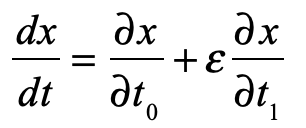
where x₀ is a slow response and acts as an envelope function for x₁ that is the fast response. The total differential is

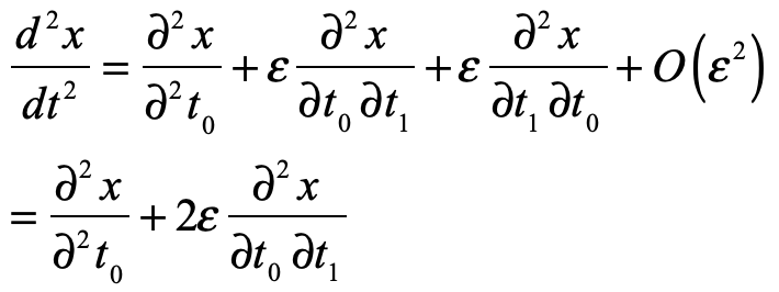
Similarly, to obtain a second derivative

Therefore, the vdP equation in terms of x₀ and x₁ is

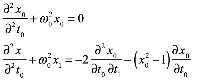
to lowest order. Now separate the orders to zeroth and first orders in ε, respectively,

Solve the first equation (a simple harmonic oscillator)

and plug the solution it into the right-hand side of the second equation to give

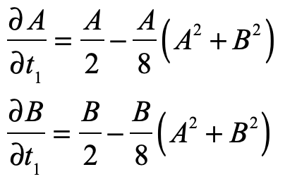
The key to secular perturbation theory is to confine dynamics to their own time scales. In other words, the slow dynamics provide the envelope that modulates the fast carrier frequency. The envelope dynamics are contained in the time dependence of the coefficients A and B. Furthermore, the dynamics of x₁ should be a homogeneous function of time, which requires each term in the last equation to be zero. Therefore, the dynamical equations for the envelope functions are

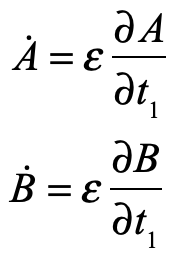
These can be transformed into polar coordinates. Because the envelope functions do not depend on the slow time scale, the time derivatives are

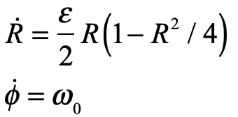
With these expressions, the slow dynamics become

where the angular velocity in the fast variable is equal to zero, leaving only the angular velocity of the unperturbed oscillator. (This is analogous to the rotating wave approximation (RWA) in optics, and also equivalent to studying the dynamics in the rotating frame of the unperturbed oscillator.)

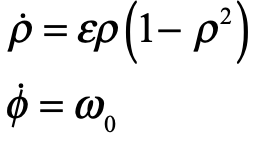
Making a final substitution ρ = R/2 gives a very simple set of dynamical equations

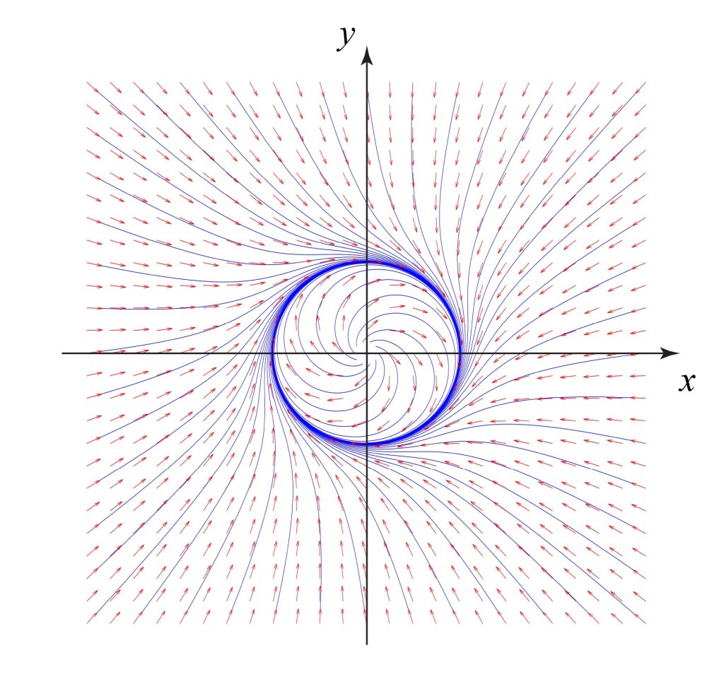
These final equations capture the essential properties of the relaxation of the dynamics to the limit cycle. To lowest order (when the gain is weak) the angular frequency is unaffected, and the system oscillates at the natural frequency. The amplitude of the limit cycle equals 1. A deviation in the amplitude from 1 decays slowly back to the limit cycle making it a stable fixed point in the radial dynamics. This analysis has converted the two-dimensional dynamics of the autonomous oscillator to a simple one-dimensional dynamics with a stable fixed point on the radius variable. The phase-space portrait of this simplified autonomous oscillator is shown in Fig. 3. What could be simpler? This simplified autonomous oscillator can be found as a fundamental element of many complex systems.

Fig. 3 The state-space diagram of the simplified autonomous oscillator. Initial conditions relax onto the limit cycle. (Reprinted from Introduction to Modern Dynamics (Oxford, 2019) on pg. 8)

Orbiting Photons around a Black Hole

The physics of a path of light passing a gravitating body is one of the hardest concepts to understand in General Relativity, but it is also one of the easiest. It is hard because there can be no force of gravity on light even though the path of a photon bends as it passes a gravitating body. It is easy, because the photon is following the simplest possible path—a geodesic equation for force-free motion.

This blog picks up where my last blog left off, having there defined the geodesic equation and presenting the Schwarzschild metric. With those two equations in hand, we could simply solve for the null geodesics (a null geodesic is the path of a light beam through a manifold). But there turns out to be a simpler approach that Einstein came up with himself (he never did like doing things the hard way). He just had to sacrifice the fundamental postulate that he used to explain everything about Special Relativity.

Throwing Special Relativity Under the Bus

The fundamental postulate of Special Relativity states that the speed of light is the same for all observers. Einstein posed this postulate, then used it to derive some of the most astonishing consequences of Special Relativity—like E = mc². This postulate is at the rock core of his theory of relativity and can be viewed as one of the simplest “truths” of our reality—or at least of our spacetime.

Yet as soon as Einstein began thinking how to extend SR to a more general situation, he realized almost immediately that he would have to throw this postulate out. While the speed of light measured locally is always equal to c, the apparent speed of light observed by a distant observer (far from the gravitating body) is modified by gravitational time dilation and length contraction. This means that the apparent speed of light, as observed at a distance, varies as a function of position. From this simple conclusion Einstein derived a first estimate of the deflection of light by the Sun, though he initially was off by a factor of 2. (The full story of Einstein’s derivation of the deflection of light by the Sun and the confirmation by Eddington is in Chapter 7 of Galileo Unbound (Oxford University Press, 2018).)

The “Optics” of Gravity

The invariant element for a light path moving radially in the Schwarzschild geometry is

The apparent speed of light is then

where c(r) is always less than c, when observing it from flat space. The “refractive index” of space is defined, as for any optical material, as the ratio of the constant speed divided by the observed speed

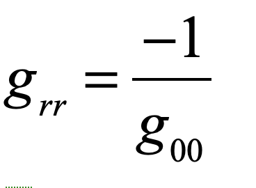
Because the Schwarzschild metric has the property

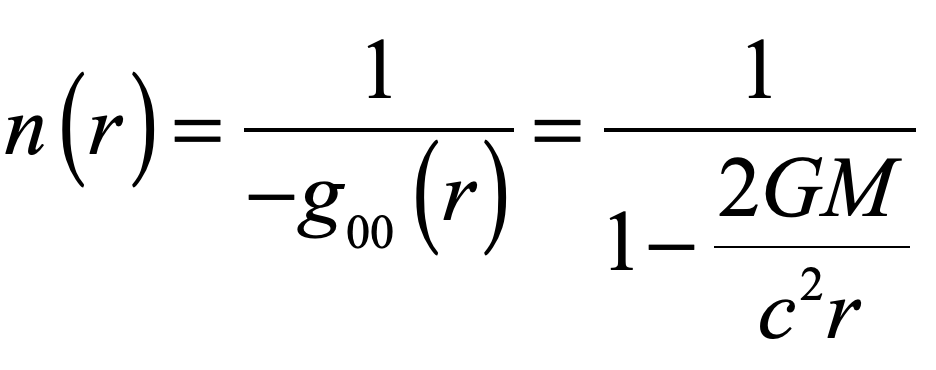
the effective refractive index of warped space-time is

with a divergence at the Schwarzschild radius.

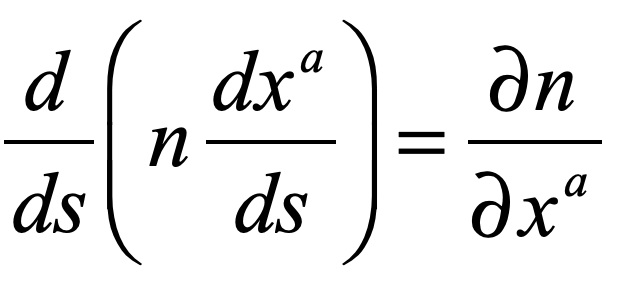
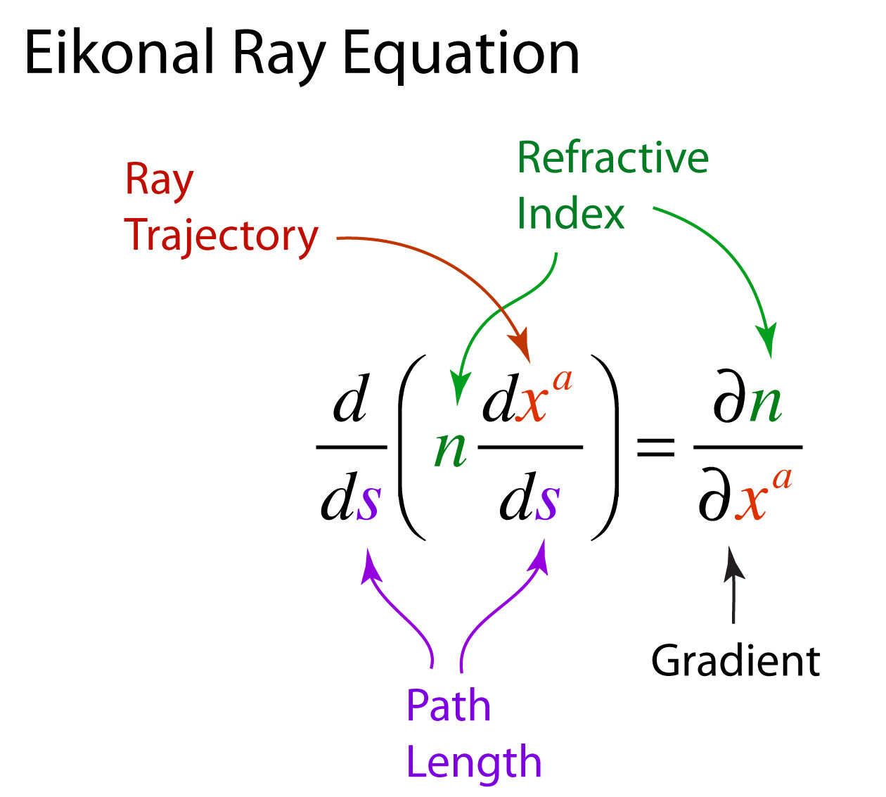
The refractive index of warped space-time in the limit of weak gravity can be used in the ray equation (also known as the Eikonal equation described in an earlier blog)

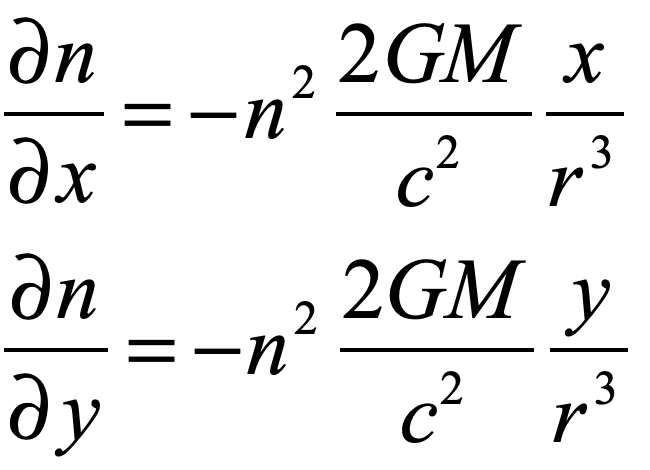
where the gradient of the refractive index of space is

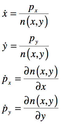
The ray equation is then a four-variable flow

These equations represent a 4-dimensional flow for a light ray confined to a plane. The trajectory of any light path is found by using an ODE solver subject to the initial conditions for the direction of the light ray. This is simple for us to do today with Python or Matlab, but it was also that could be done long before the advent of computers by early theorists of relativity like Max von Laue (1879 – 1960).

The Relativity of Max von Laue

In the Fall of 1905 in Berlin, a young German physicist by the name of Max Laue was sitting in the physics colloquium at the University listening to another Max, his doctoral supervisor Max Planck, deliver a seminar on Einstein’s new theory of relativity. Laue was struck by the simplicity of the theory, in this sense “simplistic” and hence hard to believe, but the beauty of the theory stuck with him, and he began to think through the consequences for experiments like the Fizeau experiment on partial ether drag.

Armand Hippolyte Louis Fizeau (1819 – 1896) in 1851 built one of the world’s first optical interferometers and used it to measure the speed of light inside moving fluids. At that time the speed of light was believed to be a property of the luminiferous ether, and there were several opposing theories on how light would travel inside moving matter. One theory would have the ether fully stationary, unaffected by moving matter, and hence the speed of light would be unaffected by motion. An opposite theory would have the ether fully entrained by matter and hence the speed of light in moving matter would be a simple sum of speeds. A middle theory considered that only part of the ether was dragged along with the moving matter. This was Fresnel’s partial ether drag hypothesis that he had arrived at to explain why his friend Francois Arago had not observed any contribution to stellar aberration from the motion of the Earth through the ether. When Fizeau performed his experiment, the results agreed closely with Fresnel’s drag coefficient, which seemed to settle the matter. Yet when Michelson and Morley performed their experiments of 1887, there was no evidence for partial drag.

Even after the exposition by Einstein on relativity in 1905, the disagreement of the Michelson-Morley results with Fizeau’s results was not fully reconciled until Laue showed in 1907 that the velocity addition theorem of relativity gave complete agreement with the Fizeau experiment. The velocity observed in the lab frame is found using the velocity addition theorem of special relativity. For the Fizeau experiment, water with a refractive index of n is moving with a speed v and hence the speed in the lab frame is

The difference in the speed of light between the stationary and the moving water is the difference

where the last term is precisely the Fresnel drag coefficient. This was one of the first definitive “proofs” of the validity of Einstein’s theory of relativity, and it made Laue one of relativity’s staunchest proponents. Spurred on by his success with the Fresnel drag coefficient explanation, Laue wrote the first monograph on relativity theory, publishing it in 1910.

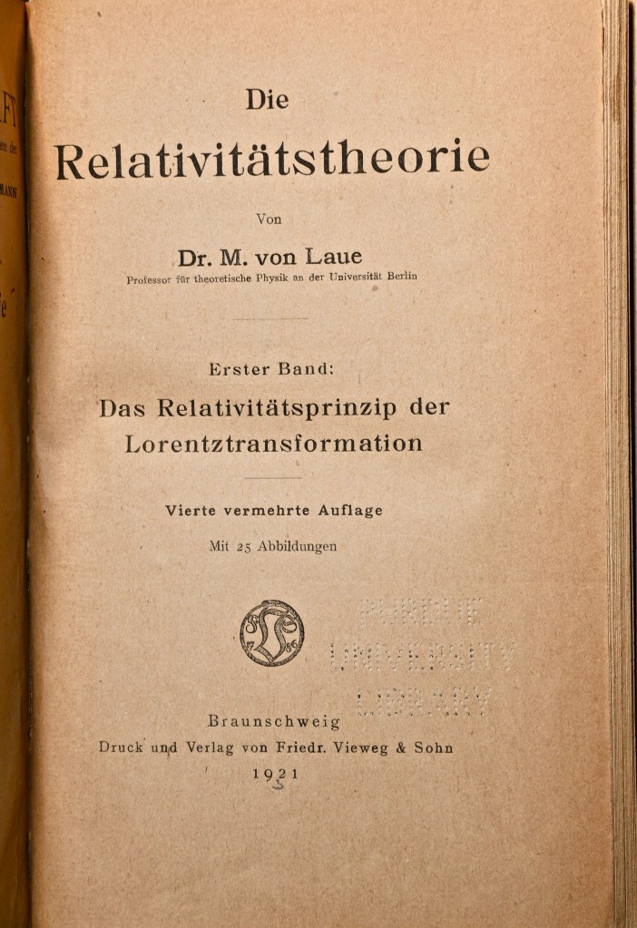
Fig. 1 Front page of von Laue’s textbook, first published in 1910, on Special Relativity (this is a 4-th edition published in 1921).

A Nobel Prize for Crystal X-ray Diffraction

In 1909 Laue became a Privatdozent under Arnold Sommerfeld (1868 – 1951) at the university in Munich. In the Spring of 1912 he was walking in the Englischer Garten on the northern edge of the city talking with Paul Ewald (1888 – 1985) who was finishing his doctorate with Sommerfed studying the structure of crystals. Ewald was considering the interaction of optical wavelength with the periodic lattice when it struck Laue that x-rays would have the kind of short wavelengths that would allow the crystal to act as a diffraction grating to produce multiple diffraction orders. Within a few weeks of that discussion, two of Sommerfeld’s students (Friedrich and Knipping) used an x-ray source and photographic film to look for the predicted diffraction spots from a copper sulfate crystal. When the film was developed, it showed a constellation of dark spots for each of the diffraction orders of the x-rays scattered from the multiple periodicities of the crystal lattice. Two years later, in 1914, Laue was awarded the Nobel prize in physics for the discovery. That same year his father was elevated to the hereditary nobility in the Prussian empire and Max Laue became Max von Laue.

Von Laue was not one to take risks, and he remained conservative in many of his interests. He was immensely respected and played important roles in the administration of German science, but his scientific contributions after receiving the Nobel Prize were only modest. Yet as the Nazis came to power in the early 1930’s, he was one of the few physicists to stand up and resist the Nazi take-over of German physics. He was especially disturbed by the plight of the Jewish physicists. In 1933 he was invited to give the keynote address at the conference of the German Physical Society in Wurzburg where he spoke out against the Nazi rejection of relativity as they branded it “Jewish science”. In his speech he likened Einstein, the target of much of the propaganda, to Galileo. He said, “No matter how great the repression, the representative of science can stand erect in the triumphant certainty that is expressed in the simple phrase: And yet it moves.” Von Laue believed that truth would hold out in the face of the proscription against relativity theory by the Nazi regime. The quote “And yet it moves” is supposed to have been muttered by Galileo just after his abjuration before the Inquisition, referring to the Earth moving around the Sun. Although the quote is famous, it is believed to be a myth.

In an odd side-note of history, von Laue sent his gold Nobel prize medal to Denmark for its safe keeping with Niels Bohr so that it would not be paraded about by the Nazi regime. Yet when the Nazis invaded Denmark, to avoid having the medals fall into the hands of the Nazis, the medal was dissolved in aqua regia by a member of Bohr’s team, George de Hevesy. The gold completely dissolved into an orange liquid that was stored in a beaker high on a shelf through the war. When Denmark was finally freed, the dissolved gold was precipitated out and a new medal was struck by the Nobel committee and re-presented to von Laue in a ceremony in 1951.

The Orbits of Light Rays

Von Laue’s interests always stayed close to the properties of light and electromagnetic radiation ever since he was introduced to the field when he studied with Woldemor Voigt at Göttingen in 1899. This interest included the theory of relativity, and only a few years after Einstein published his theory of General Relativity and Gravitation, von Laue added to his earlier textbook on relativity by writing a second volume on the general theory. The new volume was published in 1920 and included the theory of the deflection of light by gravity.

One of the very few illustrations in his second volume is of light coming into interaction with a super massive gravitational field characterized by a Schwarzschild radius. (No one at the time called it a “black hole”, nor even mentioned Schwarzschild. That terminology came much later.) He shows in the drawing, how light, if incident at just the right impact parameter, would actually loop around the object. This is the first time such a diagram appeared in print, showing the trajectory of light so strongly affected by gravity.

Fig. 2 A page from von Laue’s second volume on relativity (first published in 1920) showing the orbit of a photon around a compact mass with “gravitational cutoff” (later known as a “black hole:”). The figure is drawn semi-quantitatively, but the phenomenon was clearly understood by von Laue.

Python Code: gravlens.py

#!/usr/bin/env python3
# -*- coding: utf-8 -*-
"""
gravlens.py
Created on Tue May 28 11:50:24 2019
@author: nolte
D. D. Nolte, Introduction to Modern Dynamics: Chaos, Networks, Space and Time, 2nd ed. (Oxford,2019)
"""

import numpy as np
import matplotlib as mpl
from mpl_toolkits.mplot3d import Axes3D
from scipy import integrate
from matplotlib import pyplot as plt
from matplotlib import cm
import time
import os

plt.close('all')

def create_circle():
	circle = plt.Circle((0,0), radius= 10, color = 'black')
	return circle

def show_shape(patch):
	ax=plt.gca()
	ax.add_patch(patch)
	plt.axis('scaled')
	plt.show()
    
def refindex(x,y):
    
    A = 10
    eps = 1e-6
    
    rp0 = np.sqrt(x**2 + y**2);
        
    n = 1/(1 - A/(rp0+eps))
    fac = np.abs((1-9*(A/rp0)**2/8))   # approx correction to Eikonal
    nx = -fac*n**2*A*x/(rp0+eps)**3
    ny = -fac*n**2*A*y/(rp0+eps)**3
     
    return [n,nx,ny]

def flow_deriv(x_y_z,tspan):
    x, y, z, w = x_y_z
    
    [n,nx,ny] = refindex(x,y)
        
    yp = np.zeros(shape=(4,))
    yp[0] = z/n
    yp[1] = w/n
    yp[2] = nx
    yp[3] = ny
    
    return yp
                
for loop in range(-5,30):
    
    xstart = -100
    ystart = -2.245 + 4*loop
    print(ystart)
    
    [n,nx,ny] = refindex(xstart,ystart)


    y0 = [xstart, ystart, n, 0]

    tspan = np.linspace(1,400,2000)

    y = integrate.odeint(flow_deriv, y0, tspan)

    xx = y[1:2000,0]
    yy = y[1:2000,1]


    plt.figure(1)
    lines = plt.plot(xx,yy)
    plt.setp(lines, linewidth=1)
    plt.show()
    plt.title('Photon Orbits')
    
c = create_circle()
show_shape(c)
axes = plt.gca()
axes.set_xlim([-100,100])
axes.set_ylim([-100,100])

# Now set up a circular photon orbit
xstart = 0
ystart = 15

[n,nx,ny] = refindex(xstart,ystart)

y0 = [xstart, ystart, n, 0]

tspan = np.linspace(1,94,1000)

y = integrate.odeint(flow_deriv, y0, tspan)

xx = y[1:1000,0]
yy = y[1:1000,1]

plt.figure(1)
lines = plt.plot(xx,yy)
plt.setp(lines, linewidth=2, color = 'black')
plt.show()

One of the most striking effects of gravity on photon trajectories is the possibility for a photon to orbit a black hole in a circular orbit. This is shown in Fig. 3 as the black circular ring for a photon at a radius equal to 1.5 times the Schwarzschild radius. This radius defines what is known as the photon sphere. However, the orbit is not stable. Slight deviations will send the photon spiraling outward or inward.

The Eikonal approximation does not strictly hold under strong gravity, but the Eikonal equations with the effective refractive index of space still yield semi-quantitative behavior. In the Python code, a correction factor is used to match the theory to the circular photon orbits, while still agreeing with trajectories far from the black hole. The results of the calculation are shown in Fig. 3. For large impact parameters, the rays are deflected through a finite angle. At a critical impact parameter, near 3 times the Schwarzschild radius, the ray loops around the black hole. For smaller impact parameters, the rays are captured by the black hole.

Fig. 3 Photon orbits near a black hole calculated using the Eikonal equation and the effective refractive index of warped space. One ray, near the critical impact parameter, loops around the black hole as predicted by von Laue. The central black circle is the black hole with a Schwarzschild radius of 10 units. The black ring is the circular photon orbit at a radius 1.5 times the Schwarzschild radius.

Photons pile up around the black hole at the photon sphere. The first image ever of the photon sphere of a black hole was made earlier this year (announced April 10, 2019). The image shows the shadow of the supermassive black hole in the center of Messier 87 (M87), an elliptical galaxy 55 million light-years from Earth. This black hole is 6.5 billion times the mass of the Sun. Imaging the photosphere required eight ground-based radio telescopes placed around the globe, operating together to form a single telescope with an optical aperture the size of our planet. The resolution of such a large telescope would allow one to image a half-dollar coin on the surface of the Moon, although this telescope operates in the radio frequency range rather than the optical.

Fig. 4 Scientists have obtained the first image of a black hole, using Event Horizon Telescope observations of the center of the galaxy M87. The image shows a bright ring formed as light bends in the intense gravity around a black hole that is 6.5 billion times more massive than the Sun.

By David D. Nolte, July 29, 2019

New from Oxford University Press: Interference and the History of Light and Optics (2023)

Read Today

July 19, 2019April 11, 2026 by David D. Nolte

Getting Armstrong, Aldrin and Collins Home from the Moon: Apollo 11 and the Three-Body Problem

Fifty years ago on the 20^th of July at nearly 11 o’clock at night, my brothers and I were peering through the screen door of a very small 1960’s Shasta compact car trailer watching the TV set on the picnic table outside the trailer door. Our family was at a camp ground in southern Michigan and the mosquitos were fierce (hence why we were inside the trailer looking out through the screen). Neil Armstrong was about to be the first human to step foot on the Moon. The image on the TV was a fuzzy black and white, with barely recognizable shapes clouded even more by the dirt and dead bugs on the screen, but it is a memory etched in my mind. I was 10 years old and I was convinced that when I grew up I would visit the Moon myself, because by then Moon travel would be like flying to Europe. It didn’t turn out that way, and fifty years later it’s a struggle to even get back there.

The dangers could have become life-threatening for the crew of Apollo 11. If they miscalculated their trajectory home and had bounced off the Earth’s atmosphere, they would have become a tragic demonstration of the chaos of three-body orbits.

So maybe I won’t get to the Moon, but maybe my grandchildren will. And if they do, I hope they know something about the three-body problem in physics, because getting to and from the Moon isn’t as easy as it sounds. Apollo 11 faced real danger at several critical points on its flight plan, but all went perfectly (except overshooting their landing site and that last boulder field right before Armstrong landed). Some of those dangers became life-threatening for the crew of Apollo 13, and if they had miscalculated their trajectory home and had bounced off the Earth’s atmosphere, they would have become a tragic demonstration of the chaos of three-body orbits. In fact, their lifeless spaceship might have returned to the Moon and back to Earth over and over again, caught in an infinite chaotic web.

The complexities of trajectories in the three-body problem arise because there are too few constants of motion and too many degrees of freedom. To get an intuitive picture of how the trajectory behaves, it is best to start with a problem known as the restricted three-body problem.

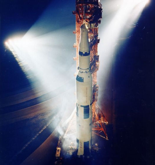
The Saturn V Booster, perhaps the pinnacle of “muscle and grit” space exploration.

The Restricted Three-Body Problem

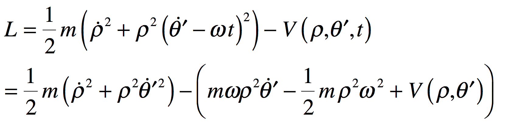
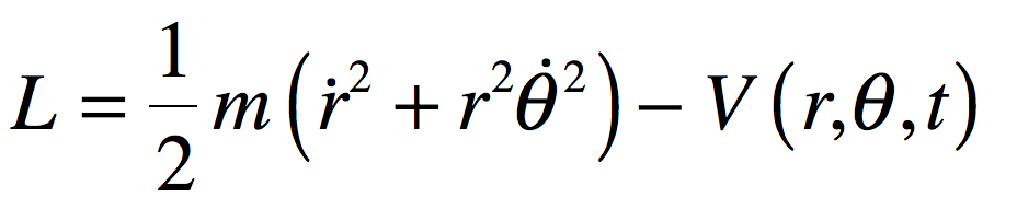
The restricted three-body problem was first considered by Leonhard Euler in 1762 (for a further discussion of the history of the three-body problem, see my Blog from July 5). For the special case of circular orbits of constant angular frequency, the motion of the third mass is described by the Lagrangian

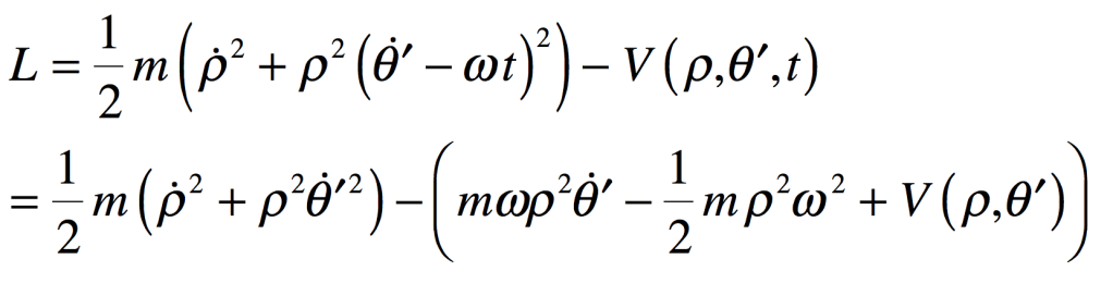
where the potential is time dependent because of the motion of the two larger masses. Lagrange approached the problem by adopting a rotating reference frame in which the two larger masses m₁ and m₂ move along the stationary line defined by their centers. The new angle variable is theta-prime. The Lagrangian in the rotating frame is

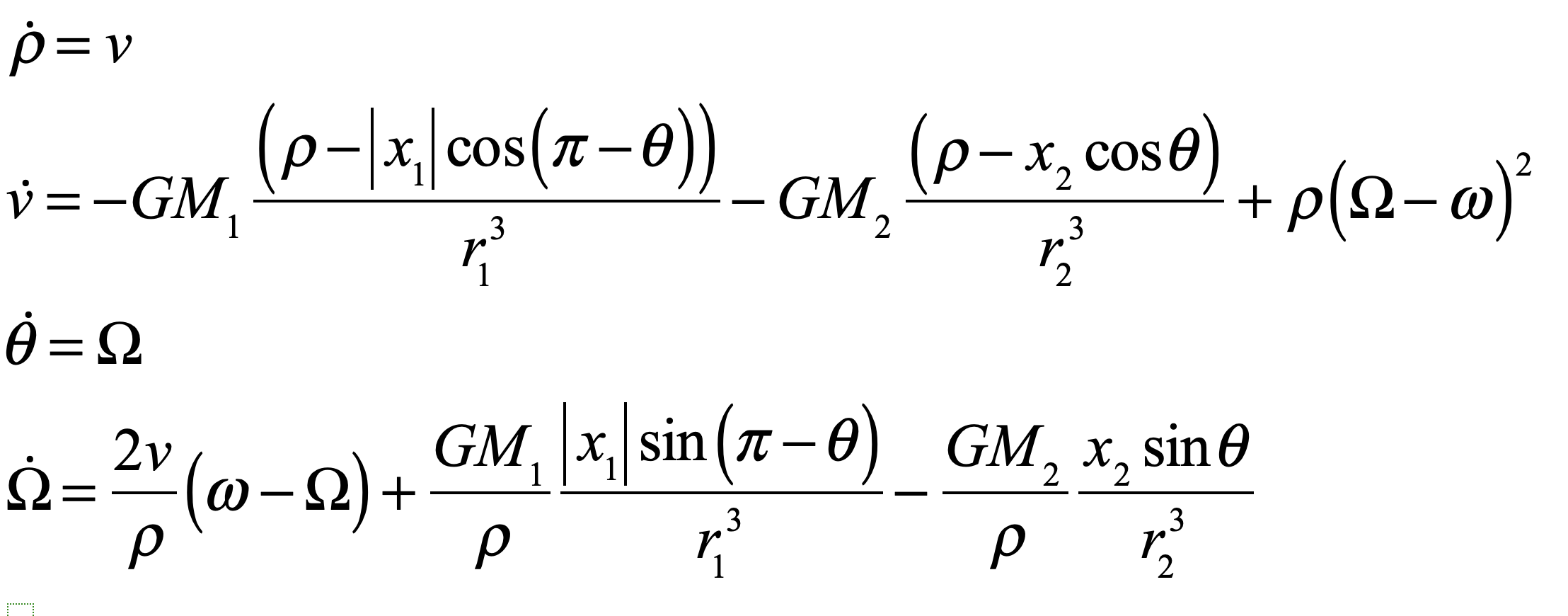
where the effective potential is now time independent. The first term in the effective potential is the Coriolis effect and the second is the centrifugal term. The dynamical flow in the plane is four dimensional, and the four-dimensional flow is

where the position vectors are in the center-of-mass frame

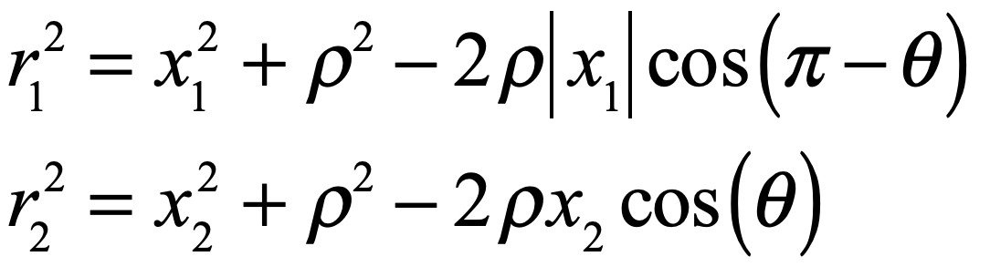
relative to the positions of the Earth and Moon (x1 and x2) in the rotating frame in which they are at rest along the x-axis.

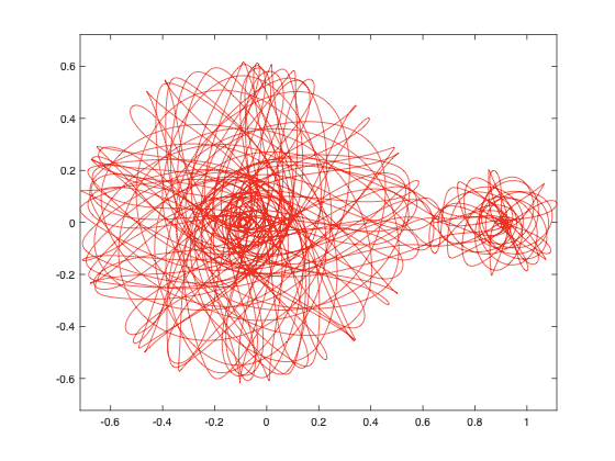
A single trajectory solved for this flow is shown in Fig. 1 for a tiny object passing back and forth chaotically between the Earth and the Moon. The object is considered to be massless, or at least so small it does not perturb the Earth-Moon system. The energy of the object was selected to allow it to pass over the potential barrier of the Lagrange-Point L1 between the Earth and the Moon. The object spends most of its time around the Earth, but now and then will get into a transfer orbit that brings it around the Moon. This would have been the fate of Apollo 11 if their last thruster burn had failed.

Fig. 1 The trajectory of a tiny object in the planar three-body problem interacting with a large mass (Earth on the left) and a small mass (Moon on the right). The energy of the trajectory allows it to pass back and forth chaotically between proximity to the Earth and proximity to the Moon. The time-duration of the simulation is approximately one decade. The envelope of the trajectories is called the “Hill region” named after one of the the first US astrophysicists George William Hill (1838-1914) who studied the 3-body problem of the Moon.

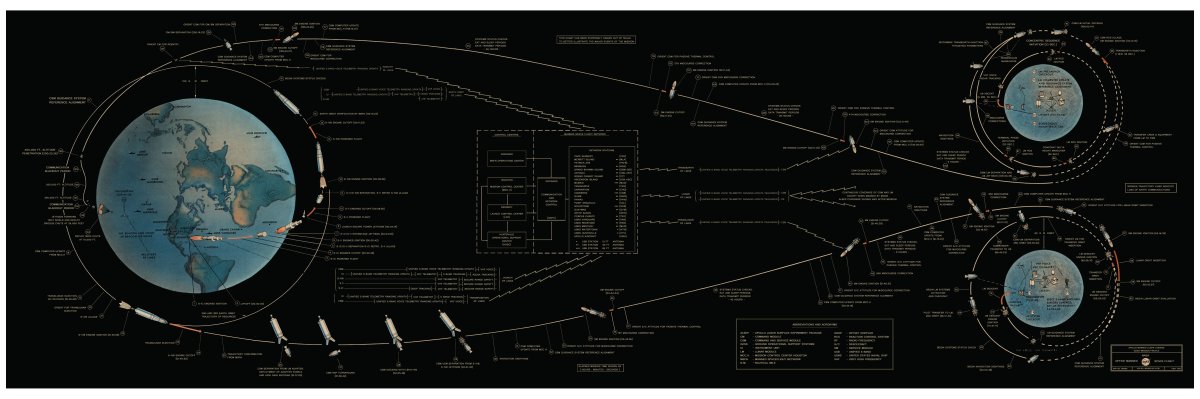
Contrast the orbit of Fig. 1 with the simple flight plan of Apollo 11 on the banner figure. The chaotic character of the three-body problem emerges for a “random” initial condition. You can play with different initial conditions in the following Python code to explore the properties of this dynamical problem. Note that in this simulation, the mass of the Moon was chosen about 8 times larger than in nature to exaggerate the effect of the Moon.

Python Code: Hill.py

(Python code on GitHub.)

#!/usr/bin/env python3
# -*- coding: utf-8 -*-
"""
Hill.py
Created on Tue May 28 11:50:24 2019
@author: nolte
D. D. Nolte, Introduction to Modern Dynamics: Chaos, Networks, Space and Time, 2nd ed. (Oxford,2019)
"""

import numpy as np
import matplotlib as mpl
from mpl_toolkits.mplot3d import Axes3D
from scipy import integrate
from matplotlib import pyplot as plt
from matplotlib import cm
import time
import os

plt.close('all')

womega = 1
R = 1
eps = 1e-6

M1 = 1     % Mass of the Earth
M2 = 1/10     % Mass of the Moon
chsi = M2/M1

x1 = -M2*R/(M1+M2)    % Earth location in rotating frame
x2 = x1 + R     % Moon location

def poten(y,c):
    
    rp0 = np.sqrt(y**2 + c**2);
    thetap0 = np.arctan(y/c);
        
    rp1 = np.sqrt(x1**2 + rp0**2 - 2*np.abs(rp0*x1)*np.cos(np.pi-thetap0));
    rp2 = np.sqrt(x2**2 + rp0**2 - 2*np.abs(rp0*x2)*np.cos(thetap0));
    V = -M1/rp1 -M2/rp2 - E;
     
    return [V]

def flow_deriv(x_y_z,tspan):
    x, y, z, w = x_y_z
    
    r1 = np.sqrt(x1**2 + x**2 - 2*np.abs(x*x1)*np.cos(np.pi-z));
    r2 = np.sqrt(x2**2 + x**2 - 2*np.abs(x*x2)*np.cos(z));
        
    yp = np.zeros(shape=(4,))
    yp[0] = y
    yp[1] = -womega**2*R**3*(np.abs(x)-np.abs(x1)*np.cos(np.pi-z))/(r1**3+eps) - womega**2*R**3*chsi*(np.abs(x)-abs(x2)*np.cos(z))/(r2**3+eps) + x*(w-womega)**2
    yp[2] = w
    yp[3] = 2*y*(womega-w)/x - womega**2*R**3*chsi*abs(x2)*np.sin(z)/(x*(r2**3+eps)) + womega**2*R**3*np.abs(x1)*np.sin(np.pi-z)/(x*(r1**3+eps))
    
    return yp
                
r0 = 0.64   % initial radius
v0 = 0.3    % initial radial speed
theta0 = 0   % initial angle
vrfrac = 1   % fraction of speed in radial versus angular directions

rp1 = np.sqrt(x1**2 + r0**2 - 2*np.abs(r0*x1)*np.cos(np.pi-theta0))
rp2 = np.sqrt(x2**2 + r0**2 - 2*np.abs(r0*x2)*np.cos(theta0))
V = -M1/rp1 - M2/rp2
T = 0.5*v0**2
E = T + V

vr = vrfrac*v0
W = (2*T - v0**2)/r0

y0 = [r0, vr, theta0, W]   % This is where you set the initial conditions

tspan = np.linspace(1,2000,20000)

y = integrate.odeint(flow_deriv, y0, tspan)

xx = y[1:20000,0]*np.cos(y[1:20000,2]);
yy = y[1:20000,0]*np.sin(y[1:20000,2]);

plt.figure(1)
lines = plt.plot(xx,yy)
plt.setp(lines, linewidth=0.5)
plt.show()

In the code, set the position and speed of the Apollo command module on lines 56-59 and put in the initial conditions on line 70. The mass of the Moon in nature is 1/81 of the mass of the Earth, which shrinks the L1 “bottleneck” to a much smaller region that you can explore to see what the fate of the Apollo missions could have been.

How to Teach General Relativity to Undergraduate Physics Majors

As a graduate student in physics at Berkeley in the 1980’s, I took General Relativity (aka GR), from Bruno Zumino, who was a world-famous physicist known as one of the originators of super-symmetry in quantum gravity (not to be confused with super-asymmetry of Cooper-Fowler Big Bang Theory fame). The class textbook was Gravitation and cosmology: principles and applications of the general theory of relativity, by Steven Weinberg, another world-famous physicist, in this case known for grand unification of the electro-weak force with electromagnetism. With so much expertise at hand, how could I fail but to absorb the simple essence of general relativity?

The answer is that I failed miserably. Somehow, I managed to pass the course, but I walked away with nothing! And it bugged me for years. What was so hard about GR? It took me almost a decade teaching undergraduate physics classes at Purdue in the 90’s before I realized that it my biggest obstacle had been language: I kept mistaking the words and terms of GR as if they were English. Words like “general covariance” and “contravariant” and “contraction” and “covariant derivative”. They sounded like English, with lots of “co” prefixes that were hard to keep straight, but they actually are part of a very different language that I call Physics-ese,

Physics-ese is a language that has lots of words that sound like English, and so you think you know what the words mean, but the words have sometimes opposite meanings than what you would guess. And the meanings of Physics-ese are precisely defined, and not something that can be left to interpretation. I learned this while teaching the intro courses to non-majors, because so many times when the students were confused, it turned out that it was because they had mistaken a textbook jargon term to be English. If you told them that the word wasn’t English, but just a token standing for a well-defined object or process, it would unshackle them from their misconceptions.

Then, in the early 00’s when I started to explore the physics of generalized trajectories related to some of my own research interests, I realized that the primary obstacle to my learning anything in the Gravitation course was Physics-ese. So this raised the question in my mind: what would it take to teach GR to undergraduate physics majors in a relatively painless manner? This is my answer.

More on this topic can be found in Chapter 11 of the textbook IMD2: Introduction to Modern Dynamics, 2^nd Edition, Oxford University Press, 2019

Trajectories as Flows

One of the culprits for my mind block learning GR was Newton himself. His ubiquitous second law, taught as F = ma, is surprisingly misleading if one wants to have a more general understanding of what a trajectory is. This is particularly the case for light paths, which can be bent by gravity, yet clearly cannot have any forces acting on them.

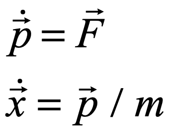
The way to fix this is subtle yet simple. First, express Newton’s second law as

which is actually closer to the way that Newton expressed the law in his Principia. In three dimensions for a single particle, these equations represent a 6-dimensional dynamical space called phase space: three coordinate dimensions and three momentum dimensions. Then generalize the vector quantities, like the position vector, to be expressed as x^a for the six dynamics variables: x, y, z, p_x, p_y, and p_z.

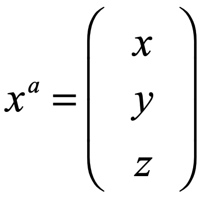
Now, as part of Physics-ese, putting the index as a superscript instead as a subscript turns out to be a useful notation when working in higher-dimensional spaces. This superscript is called a “contravariant index” which sounds like English but is uninterpretable without a Physics-ese-to-English dictionary. All “contravariant index” means is “column vector component”. In other words, x^a is just the position vector expressed as a column vector

This superscripted index is called a “contravariant” index, but seriously dude, just forget that “contravariant” word from Physics-ese and just think “index”. You already know it’s a column vector.

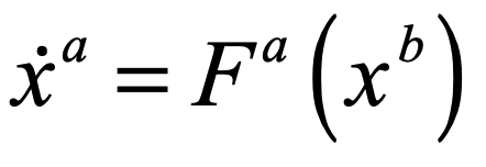
Then Newton’s second law becomes

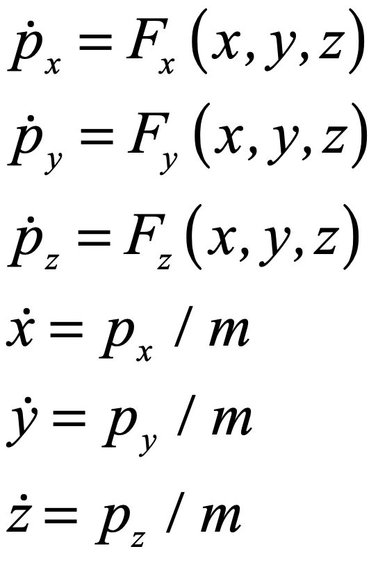
where the index a runs from 1 to 6, and the function F^a is a vector function of the dynamic variables. To spell it out, this is

so it’s a lot easier to write it in the one-line form with the index notation.

The simple index notation equation is in the standard form for what is called, in Physics-ese, a “mathematical flow”. It is an ODE that can be solved for any set of initial conditions for a given trajectory. Or a whole field of solutions can be considered in a phase-space portrait that looks like the flow lines of hydrodynamics. The phase-space portrait captures the essential physics of the system, whether it is a rock thrown off a cliff, or a photon orbiting a black hole. But to get to that second problem, it is necessary to look deeper into the way that space is described by any set of coordinates, especially if those coordinates are changing from location to location.

What’s so Fictitious about Fictitious Forces?

Freshmen physics students are routinely admonished for talking about “centrifugal” forces (rather than centripetal) when describing circular motion, usually with the statement that centrifugal forces are fictitious—only appearing to be forces when the observer is in the rotating frame. The same is said for the Coriolis force. Yet for being such a “fictitious” force, the Coriolis effect is what drives hurricanes and the colossal devastation they cause. Try telling a hurricane victim that they were wiped out by a fictitious force! Looking closer at the Coriolis force is a good way of understanding how taking derivatives of vectors leads to effects often called “fictitious”, yet it opens the door on some of the simpler techniques in the topic of differential geometry.

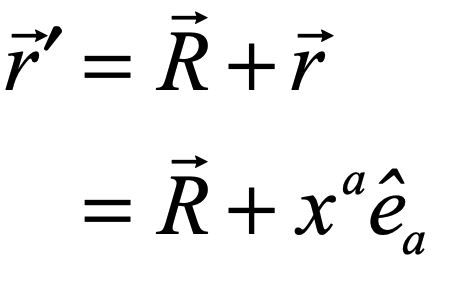
To start, consider a vector in a uniformly rotating frame. Such a frame is called “non-inertial” because of the angular acceleration associated with the uniform rotation. For an observer in the rotating frame, vectors are attached to the frame, like pinning them down to the coordinate axes, but the axes themselves are changing in time (when viewed by an external observer in a fixed frame). If the primed frame is the external fixed frame, then a position in the rotating frame is

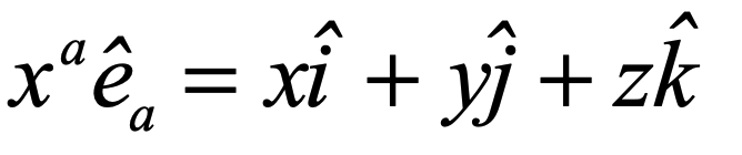
where R is the position vector of the origin of the rotating frame and r is the position in the rotating frame relative to the origin. The funny notation on the last term is called in Physics-ese a “contraction”, but it is just a simple inner product, or dot product, between the components of the position vector and the basis vectors. A basis vector is like the old-fashioned i, j, k of vector calculus indicating unit basis vectors pointing along the x, y and z axes. The format with one index up and one down in the product means to do a summation. This is known as the Einstein summation convention, so it’s just

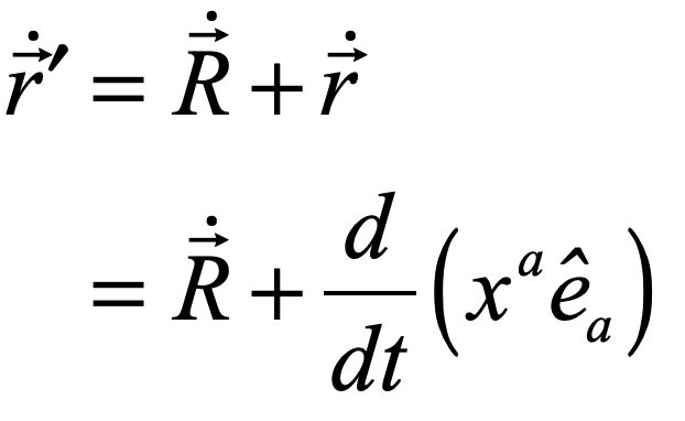
Taking the time derivative of the position vector gives

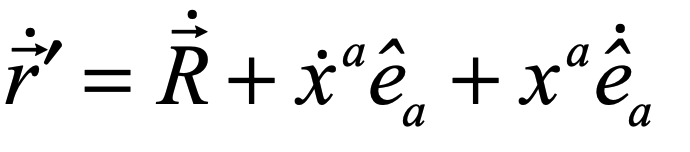
and by the chain rule this must be

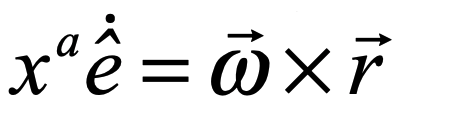
where the last term has a time derivative of a basis vector. This is non-zero because in the rotating frame the basis vector is changing orientation in time. This term is non-inertial and can be shown fairly easily (see IMD2 Chapter 1) to be

which is where the centrifugal force comes from. This shows how a so-called fictitious force arises from a derivative of a basis vector. The fascinating point of this is that in GR, the force of gravity arises in almost the same way, making it tempting to call gravity a fictitious force, despite the fact that it can kill you if you fall out a window. The question is, how does gravity arise from simple derivatives of basis vectors?

The Geodesic Equation

To teach GR to undergraduates, you cannot expect them to have taken a course in differential geometry, because most of them just don’t have the time in their schedule to take such an advanced mathematics course. In addition, there is far more taught in differential geometry than is needed to make progress in GR. So the simple approach is to teach what they need to understand GR with as little differential geometry as possible, expressed with clear English-to-Physics-ese translations.

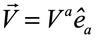
For example, consider the partial derivative of a vector expressed in index notation as

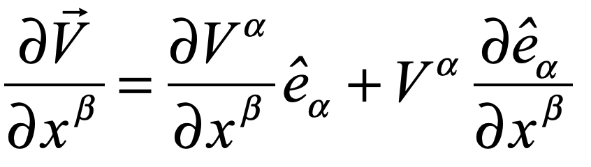
Taking the partial derivative, using the always-necessary chain rule, is

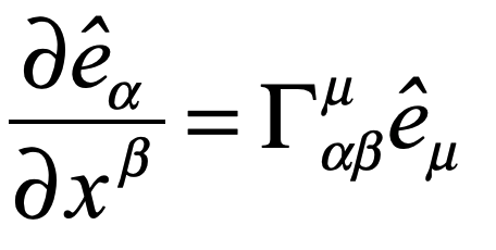
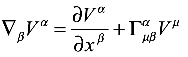
where the second term is just like the extra time-derivative term that showed up in the derivation of the Coriolis force. The basis vector of a general coordinate system may change size and orientation as a function of position, so this derivative is not in general zero. Because the derivative of a basis vector is so central to the ideas of GR, they are given their own symbol. It is

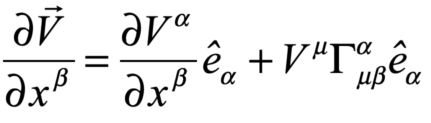
where the new “Gamma” symbol is called a Christoffel symbol. It has lots of indexes, both up and down, which looks daunting, but it can be interpreted as the beta-th derivative of the alpha-th component of the mu-th basis vector. The partial derivative is now

For those of you who noticed that some of the indexes flipped from alpha to mu and vice versa, you’re right! Swapping repeated indexes in these “contractions” is allowed and helps make derivations a lot easier, which is probably why Einstein invented this notation in the first place.

The last step in taking a partial derivative of a vector is to isolate a single vector component V^a as

where a new symbol, the del-operator has been introduced. This del-operator is known as the “covariant derivative” of the vector component. Again, forget the “covariant” part and just think “gradient”. Namely, taking the gradient of a vector in general includes changes in the vector component as well as changes in the basis vector.

Now that you know how to take the partial derivative of a vector using Christoffel symbols, you are ready to generate the central equation of General Relativity: The geodesic equation.

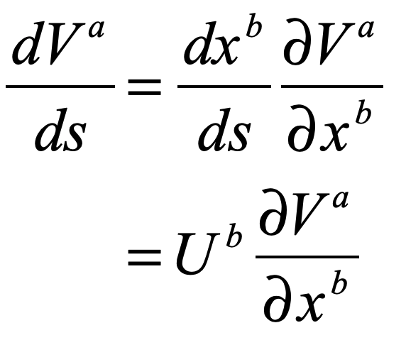
Everyone knows that a geodesic is the shortest path between two points, like a great circle route on the globe. But it also turns out to be the straightest path, which can be derived using an idea known as “parallel transport”. To start, consider transporting a vector along a curve in a flat metric. The equation describing this process is

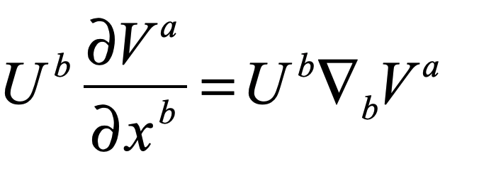
Because the Christoffel symbols are zero in a flat space, the covariant derivative and the partial derivative are equal, giving

If the vector is transported parallel to itself, then there is no change in V along the curve, so that

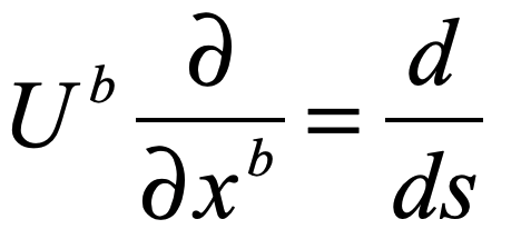
Finally, recognizing

and substituting this in gives

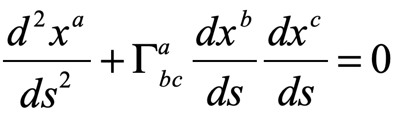
This is the geodesic equation!

Fig. 1 The geodesic equation of motion is for force-free motion through a metric space. The curvature of the trajectory is analogous to acceleration, and the generalized gradient is analogous to a force. The geodesic equation is the “F = ma” of GR.

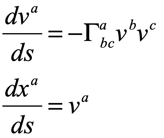
Putting this in the standard form of a flow gives the geodesic flow equations

The flow defines an ordinary differential equation that defines a curve that carries its own tangent vector onto itself. The curve is parameterized by a parameter s that can be identified with path length. It is the central equation of GR, because it describes how an object follows a force-free trajectory, like free fall, in any general coordinate system. It can be applied to simple problems like the Coriolis effect, or it can be applied to seemingly difficult problems, like the trajectory of a light path past a black hole.

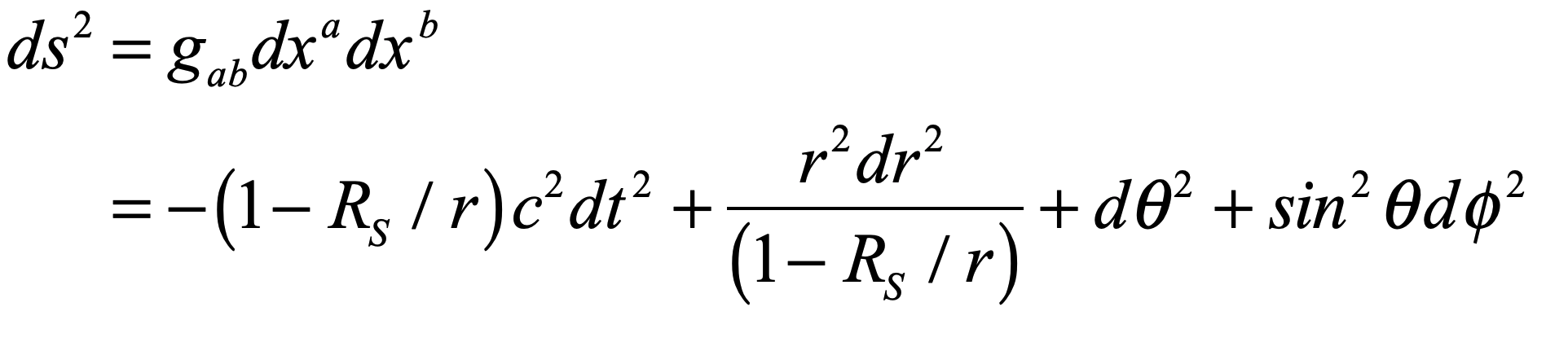
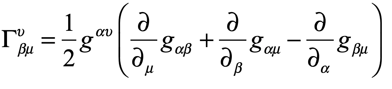
The Metric Connection

Arriving at the geodesic equation is a major accomplishment, and you have done it in just a few pages of this blog. But there is still an important missing piece before we are doing General Relativity of gravitation. We need to connect the Christoffel symbol in the geodesic equation to the warping of space-time around a gravitating object.

The warping of space-time by matter and energy is another central piece of GR and is often the central focus of a graduate-level course on the subject. This part of GR does have its challenges leading up to Einstein’s Field Equations that explain how matter makes space bend. But at an undergraduate level, it is sufficient to just describe the bent coordinates as a starting point, then use the geodesic equation to solve for so many of the cool effects of black holes.

So, stating the way that matter bends space-time is as simple as writing down the length element for the Schwarzschild metric of a spherical gravitating mass as

where R_S = GM/c² is the Schwarzschild radius. (The connection between the metric tensor g_ab and the Christoffel symbol can be found in Chapter 11 of IMD2.) It takes only a little work to find that

This means that if we have the Schwarzschild metric, all we have to do is take first partial derivatives and we will arrive at the Christoffel symbols that go into the geodesic equation. Solving for any type of force-free trajectory is then just a matter of solving ODEs with initial conditions (performed routinely with numerical ODE solvers in Python, Matlab, Mathematica, etc.).

The first problem we will tackle using the geodesic equation is the deflection of light by gravity. This is the quintessential problem of GR because there cannot be any gravitational force on a photon, yet the path of the photon surely must bend in the presence of gravity. This is possible through the geodesic motion of the photon through warped space time. I’ll take up this problem in my next Blog.

July 5, 2019July 7, 2019 by David D. Nolte

The Three-Body Problem, Longitude at Sea, and Lagrange’s Points

When Newton developed his theory of universal gravitation, the first problem he tackled was Kepler’s elliptical orbits of the planets around the sun, and he succeeded beyond compare. The second problem he tackled was of more practical importance than the tracks of distant planets, namely the path of the Earth’s own moon, and he was never satisfied.

Newton’s Principia and the Problem of Longitude

Measuring the precise location of the moon at very exact times against the backdrop of the celestial sphere was a method for ships at sea to find their longitude. Yet the moon’s orbit around the Earth is irregular, and Newton recognized that because gravity was universal, every planet exerted a force on each other, and the moon was being tugged upon by the sun as well as by the Earth.

Newton’s attempt with the Moon was his last significant scientific endeavor

In Propositions 65 and 66 of Book 1 of the Principia, Newton applied his new theory to attempt to pin down the moon’s trajectory, but was thwarted by the complexity of the three bodies of the Earth-Moon-Sun system. For instance, the force of the sun on the moon is greater than the force of the Earth on the moon, which raised the question of why the moon continued to circle the Earth rather than being pulled away to the sun. Newton correctly recognized that it was the Earth-moon system that was in orbit around the sun, and hence the sun caused only a perturbation on the Moon’s orbit around the Earth. However, because the Moon’s orbit is approximately elliptical, the Sun’s pull on the Moon is not constant as it swings around in its orbit, and Newton only succeeded in making estimates of the perturbation.

Unsatisfied with his results in the Principia, Newton tried again, beginning in the summer of 1694, but the problem was to too great even for him. In 1702 he published his research, as far as he was able to take it, on the orbital trajectory of the Moon. He could pin down the motion to within 10 arc minutes, but this was not accurate enough for reliable navigation, representing an uncertainty of over 10 kilometers at sea—error enough to run aground at night on unseen shoals. Newton’s attempt with the Moon was his last significant scientific endeavor, and afterwards this great scientist withdrew into administrative activities and other occult interests that consumed his remaining time.

Race for the Moon

The importance of the Moon for navigation was too pressing to ignore, and in the 1740’s a heated competition to be the first to pin down the Moon’s motion developed among three of the leading mathematicians of the day—Leonhard Euler, Jean Le Rond D’Alembert and Alexis Clairaut—who began attacking the lunar problem and each other [1]. Euler in 1736 had published the first textbook on dynamics that used the calculus, and Clairaut had recently returned from Lapland with Maupertuis. D’Alembert, for his part, had placed dynamics on a firm physical foundation with his 1743 textbook. Euler was first to publish with a lunar table in 1746, but there remained problems in his theory that frustrated his attempt at attaining the required level of accuracy.

At nearly the same time Clairaut and D’Alembert revisited Newton’s foiled lunar theory and found additional terms in the perturbation expansion that Newton had neglected. They rushed to beat each other into print, but Clairaut was distracted by a prize competition for the most accurate lunar theory, announced by the Russian Academy of Sciences and refereed by Euler, while D’Alembert ignored the competition, certain that Euler would rule in favor of Clairaut. Clairaut won the prize, but D’Alembert beat him into print.

The rivalry over the moon did not end there. Clairaut continued to improve lunar tables by combining theory and observation, while D’Alembert remained more purely theoretical. A growing animosity between Clairaut and D’Alembert spilled out into the public eye and became a daily topic of conversation in the Paris salons. The difference in their approaches matched the difference in their personalities, with the more flamboyant and pragmatic Clairaut disdaining the purist approach and philosophy of D’Alembert. Clairaut succeeded in publishing improved lunar theory and tables in 1752, followed by Euler in 1753, while D’Alembert’s interests were drawn away towards his activities for Diderot’s Encyclopedia.

The battle over the Moon in the late 1740’s was carried out on the battlefield of perturbation theory. To lowest order, the orbit of the Moon around the Earth is a Keplerian ellipse, and the effect of the Sun, though creating problems for the use of the Moon for navigation, produces only a small modification—a perturbation—of its overall motion. Within a decade or two, the accuracy of perturbation theory calculations, combined with empirical observations, had improved to the point that accurate lunar tables had sufficient accuracy to allow ships to locate their longitude to within a kilometer at sea. The most accurate tables were made by Tobias Mayer, who was awarded posthumously a prize of 3000 pounds by the British Parliament in 1763 for the determination of longitude at sea. Euler received 300 pounds for helping Mayer with his calculations. This was the same prize that was coveted by the famous clockmaker John Harrison and depicted so brilliantly in Dava Sobel’s Longitude (1995).

Lagrange Points

Several years later in 1772 Lagrange discovered an interesting special solution to the planar three-body problem with three massive points each executing an elliptic orbit around the center of mass of the system, but configured such that their positions always coincided with the vertices of an equilateral triangle [2]. He found a more important special solution in the restricted three-body problem that emerged when a massless third body was found to have two stable equilibrium points in the combined gravitational potentials of two massive bodies. These two stable equilibrium points are known as the L4 and L5 Lagrange points. Small objects can orbit these points, and in the Sun-Jupiter system these points are occupied by the Trojan asteroids. Similarly stable Lagrange points exist in the Earth-Moon system where space stations or satellites could be parked.

For the special case of circular orbits of constant angular frequency w, the motion of the third mass is described by the Lagrangian

where the effective potential is now time independent. The first term in the effective potential is the Coriolis effect and the second is the centrifugal term.

Fig. Effective potential for the planar three-body problem and the five Lagrange points where the gradient of the effective potential equals zero. The Lagrange points are displayed on a horizontal cross section of the potential energy shown with equipotential lines. The large circle in the center is the Sun. The smaller circle on the right is a Jupiter-like planet. The points L1, L2 and L3 are each saddle-point equilibria positions and hence unstable. The points L4 and L5 are stable points that can collect small masses that orbit these Lagrange points.

The effective potential is shown in the figure for m₃ = 10m₂. There are five locations where the gradient of the effective potential equals zero. The point L1 is the equilibrium position between the two larger masses. The points L2 and L3 are at positions where the centrifugal force balances the gravitational attraction to the two larger masses. These are also the points that separate local orbits around a single mass from global orbits that orbit the two-body system. The last two Lagrange points at L4 and L5 are at one of the vertices of an equilateral triangle, with the other two vertices at the positions of the larger masses. The first three Lagrange points are saddle points. The last two are at maxima of the effective potential.

L1, lies between Earth and the sun at about 1 million miles from Earth. L1 gets an uninterrupted view of the sun, and is currently occupied by the Solar and Heliospheric Observatory (SOHO) and the Deep Space Climate Observatory. L2 also lies a million miles from Earth, but in the opposite direction of the sun. At this point, with the Earth, moon and sun behind it, a spacecraft can get a clear view of deep space. NASA’s Wilkinson Microwave Anisotropy Probe (WMAP) is currently at this spot measuring the cosmic background radiation left over from the Big Bang. The James Webb Space Telescope will move into this region in 2021.

[1] Gutzwiller, M. C. (1998). “Moon-Earth-Sun: The oldest three-body problem.” Reviews of Modern Physics 70(2): 589-639.

[2] J.L. Lagrange Essai sur le problème des trois corps, 1772, Oeuvres tome 6

June 16, 2019June 1, 2023 by David D. Nolte

Vladimir Arnold’s Cat Map

The 1960’s are known as a time of cultural revolution, but perhaps less known was the revolution that occurred in the science of dynamics. Three towering figures of that revolution were Stephen Smale (1930 – ) at Berkeley, Andrey Kolmogorov (1903 – 1987) in Moscow and his student Vladimir Arnold (1937 – 2010). Arnold was only 20 years old in 1957 when he solved Hilbert’s thirteenth problem (that any continuous function of several variables can be constructed with a finite number of two-variable functions). Only a few years later his work on the problem of small denominators in dynamical systems provided the finishing touches on the long elusive explanation of the stability of the solar system (the problem for which Poincaré won the King Oscar Prize in mathematics in 1889 when he discovered chaotic dynamics ). This theory is known as KAM-theory, using the first initials of the names of Kolmogorov, Arnold and Moser [1]. Building on his breakthrough in celestial mechanics, Arnold’s work through the 1960’s remade the theory of Hamiltonian systems, creating a shift in perspective that has permanently altered how physicists look at dynamical systems.

Hamiltonian Physics on a Torus

Traditionally, Hamiltonian physics is associated with systems of inertial objects that conserve the sum of kinetic and potential energy, in other words, conservative non-dissipative systems. But a modern view (after Arnold) of Hamiltonian systems sees them as hyperdimensional mathematical mappings that conserve volume. The space that these mappings inhabit is phase space, and the conservation of phase-space volume is known as Liouville’s Theorem [2]. The geometry of phase space is called symplectic geometry, and the universal position that symplectic geometry now holds in the physics of Hamiltonian mechanics is largely due to Arnold’s textbook Mathematical Methods of Classical Mechanics (1974, English translation 1978) [3]. Arnold’s famous quote from that text is “Hamiltonian mechanics is geometry in phase space”.

One of the striking aspects of this textbook is the reduction of phase-space geometry to the geometry of a hyperdimensional torus for a large number of Hamiltonian systems. If there are as many conserved quantities as there are degrees of freedom in a Hamiltonian system, then the system is called “integrable” (because you can integrated the equations of motion to find a constant of the motion). Then it is possible to map the physics onto a hyperdimensional torus through the transformation of dynamical coordinates into what are known as “action-angle” coordinates [4]. Each independent angle has an associated action that is conserved during the motion of the system. The periodicity of the dynamical angle coordinate makes it possible to identify it with the angular coordinate of a multi-dimensional torus. Therefore, every integrable Hamiltonian system can be mapped to motion on a multi-dimensional torus (one dimension for each degree of freedom of the system).

Actually, integrable Hamiltonian systems are among the most boring dynamical systems you can imagine. They literally just go in circles (around the torus). But as soon as you add a small perturbation that cannot be integrated they produce some of the most complex and beautiful patterns of all dynamical systems. It was Arnold’s focus on motions on a torus, and perturbations that shift the dynamics off the torus, that led him to propose a simple mapping that captured the essence of Hamiltonian chaos.

The Arnold Cat Map

Motion on a two-dimensional torus is defined by two angles, and trajectories on a two-dimensional torus are simple helixes. If the periodicities of the motion in the two angles have an integer ratio, the helix repeats itself. However, if the ratio of periods (also known as the winding number) is irrational, then the helix never repeats and passes arbitrarily closely to any point on the surface of the torus. This last case leads to an “ergodic” system, which is a term introduced by Boltzmann to describe a physical system whose trajectory fills phase space. The behavior of a helix for rational or irrational winding number is not terribly interesting. It’s just an orbit going in circles like an integrable Hamiltonian system. The helix can never even cross itself.

However, if you could add a new dimension to the torus (or add a new degree of freedom to the dynamical system), then the helix could pass over or under itself by moving into the new dimension. By weaving around itself, a trajectory can become chaotic, and the set of many trajectories can become as mixed up as a bowl of spaghetti. This can be a little hard to visualize, especially in higher dimensions, but Arnold thought of a very simple mathematical mapping that captures the essential motion on a torus, preserving volume as required for a Hamiltonian system, but with the ability for regions to become all mixed up, just like trajectories in a nonintegrable Hamiltonian system.

A unit square is isomorphic to a two-dimensional torus. This means that there is a one-to-one mapping of each point on the unit square to each point on the surface of a torus. Imagine taking a sheet of paper and forming a tube out of it. One of the dimensions of the sheet of paper is now an angle coordinate that is cyclic, going around the circumference of the tube. Now if the sheet of paper is flexible (like it is made of thin rubber) you can bend the tube around and connect the top of the tube with the bottom, like a bicycle inner tube. The other dimension of the sheet of paper is now also an angle coordinate that is cyclic. In this way a flat sheet is converted (with some bending) into a torus.

Arnold’s key idea was to create a transformation that takes the torus into itself, preserving volume, yet including the ability for regions to pass around each other. Arnold accomplished this with the simple map

where the modulus 1 takes the unit square into itself. This transformation can also be expressed as a matrix

followed by taking modulus 1. The transformation matrix is called a Floquet matrix, and the determinant of the matrix is equal to unity, which ensures that volume is conserved.

Arnold decided to illustrate this mapping by using a crude image of the face of a cat (See Fig. 1). Successive applications of the transformation stretch and shear the cat, which is then folded back into the unit square. The stretching and folding preserve the volume, but the image becomes all mixed up, just like mixing in a chaotic Hamiltonian system, or like an immiscible dye in water that is stirred.

Fig. 1 Arnold’s illustration of his cat map from pg. 6 of V. I. Arnold and A. Avez, *Ergodic Problems of Classical Mechanics* (Benjamin, 1968) [5]

Fig. 2 Arnold Cat Map operation is an iterated succession of stretching with shear of a unit square, and translation back to the unit square. The mapping preserves and mixes areas, and is invertible.

Recurrence

When the transformation matrix is applied to continuous values, it produces a continuous range of transformed values that become thinner and thinner until the unit square is uniformly mixed. However, if the unit square is discrete, made up of pixels, then something very different happens (see Fig. 3). The image of the cat in this case is composed of a 50×50 array of pixels. For early iterations, the image becomes stretched and mixed, but at iteration 50 there are 4 low-resolution upside-down versions of the cat, and at iteration 75 the cat fully reforms, but is upside-down. Continuing on, the cat eventually reappears fully reformed and upright at iteration 150. Therefore, the discrete case displays a recurrence and the mapping is periodic. Calculating the period of the cat map on lattices can lead to interesting patterns, especially if the lattice is composed of prime numbers [6].

The Cat Map and the Golden Mean

The golden mean, or the golden ratio, 1.618033988749895 is never far away when working with Hamiltonian systems. Because the golden mean is the “most irrational” of all irrational numbers, it plays an essential role in KAM theory on the stability of the solar system. In the case of Arnold’s cat map, it pops up its head in several ways. For instance, the transformation matrix has eigenvalues

with the remarkable property that

which guarantees conservation of area.

Selected V. I. Arnold Publications

Arnold, V. I. “FUNCTIONS OF 3 VARIABLES.” Doklady Akademii Nauk Sssr 114(4): 679-681. (1957)

Arnold, V. I. “GENERATION OF QUASI-PERIODIC MOTION FROM A FAMILY OF PERIODIC MOTIONS.” Doklady Akademii Nauk Sssr 138(1): 13-&. (1961)

Arnold, V. I. “STABILITY OF EQUILIBRIUM POSITION OF A HAMILTONIAN SYSTEM OF ORDINARY DIFFERENTIAL EQUATIONS IN GENERAL ELLIPTIC CASE.” Doklady Akademii Nauk Sssr 137(2): 255-&. (1961)

Arnold, V. I. “BEHAVIOUR OF AN ADIABATIC INVARIANT WHEN HAMILTONS FUNCTION IS UNDERGOING A SLOW PERIODIC VARIATION.” Doklady Akademii Nauk Sssr 142(4): 758-&. (1962)

Arnold, V. I. “CLASSICAL THEORY OF PERTURBATIONS AND PROBLEM OF STABILITY OF PLANETARY SYSTEMS.” Doklady Akademii Nauk Sssr 145(3): 487-&. (1962)

Arnold, V. I. “BEHAVIOUR OF AN ADIABATIC INVARIANT WHEN HAMILTONS FUNCTION IS UNDERGOING A SLOW PERIODIC VARIATION.” Doklady Akademii Nauk Sssr 142(4): 758-&. (1962)

Arnold, V. I. and Y. G. Sinai. “SMALL PERTURBATIONS OF AUTHOMORPHISMS OF A TORE.” Doklady Akademii Nauk Sssr 144(4): 695-&. (1962)

Arnold, V. I. “Small denominators and problems of the stability of motion in classical and celestial mechanics (in Russian).” Usp. Mat. Nauk. 18: 91-192. (1963)

Arnold, V. I. and A. L. Krylov. “UNIFORM DISTRIBUTION OF POINTS ON A SPHERE AND SOME ERGODIC PROPERTIES OF SOLUTIONS TO LINEAR ORDINARY DIFFERENTIAL EQUATIONS IN COMPLEX REGION.” Doklady Akademii Nauk Sssr 148(1): 9-&. (1963)

Arnold, V. I. “INSTABILITY OF DYNAMICAL SYSTEMS WITH MANY DEGREES OF FREEDOM.” Doklady Akademii Nauk Sssr 156(1): 9-&. (1964)

Arnold, V. “SUR UNE PROPRIETE TOPOLOGIQUE DES APPLICATIONS GLOBALEMENT CANONIQUES DE LA MECANIQUE CLASSIQUE.” Comptes Rendus Hebdomadaires Des Seances De L Academie Des Sciences 261(19): 3719-&. (1965)

Arnold, V. I. “APPLICABILITY CONDITIONS AND ERROR ESTIMATION BY AVERAGING FOR SYSTEMS WHICH GO THROUGH RESONANCES IN COURSE OF EVOLUTION.” Doklady Akademii Nauk Sssr 161(1): 9-&. (1965)

Bibliography

[1] Dumas, H. S. The KAM Story: A friendly introduction to the content, history and significance of Classical Kolmogorov-Arnold-Moser Theory, World Scientific. (2014)

[2] See Chapter 6, “The Tangled Tale of Phase Space” in Galileo Unbound (D. D. Nolte, Oxford University Press, 2018)

[3] V. I. Arnold, Mathematical Methods of Classical Mechanics (Nauk 1974, English translation Springer 1978)

[4] See Chapter 3, “Hamiltonian Dynamics and Phase Space” in Introduction to Modern Dynamics, 2nd ed. (D. D. Nolte, Oxford University Press, 2019)

[5] V. I. Arnold and A. Avez, Ergodic Problems of Classical Mechanics (Benjamin, 1968)

[6] Gaspari, G. “THE ARNOLD CAT MAP ON PRIME LATTICES.” Physica D-Nonlinear Phenomena 73(4): 352-372. (1994)

May 30, 2019November 14, 2023 by David D. Nolte

The Iconic Eikonal and the Optical Path

Nature loves the path of steepest descent. Place a ball on a smooth curved surface and release it, and it will instantansouly accelerate in the direction of steepest descent. Shoot a laser beam from an oblique angle onto a piece of glass to hit a target inside, and the path taken by the beam is the only path that decreases the distance to the target in the shortest time. Diffract a stream of electrons from the surface of a crystal, and quantum detection events are greatest at the positions where the troughs and peaks of the deBroglie waves converge the most. The first example is Newton’s second law. The second example is Fermat’s principle and Snell’s Law. The third example is Feynman’s path-integral formulation of quantum mechanics. They all share in common a minimization principle—the principle of least action—that the path of a dynamical system is the one that minimizes a property known as “action”.

The Eikonal Equation is the “F = ma” of ray optics. It’s solutions describe the paths of light rays through complicated media.

The principle of least action, first proposed by the French physicist Maupertuis through mechanical analogy, became a principle of Lagrangian mechanics in the hands of Lagrange, but was still restricted to mechanical systems of particles. The principle was generalized forty years later by Hamilton, who began by considering the propagation of light waves, and ended by transforming mechanics into a study of pure geometry divorced from forces and inertia. Optics played a key role in the development of mechanics, and mechanics returned the favor by giving optics the Eikonal Equation. The Eikonal Equation is the “F = ma” of ray optics. It’s solutions describe the paths of light rays through complicated media.

Malus’ Theorem

Anyone who has taken a course in optics knows that Étienne-Louis Malus (1775-1812) discovered the polarization of light, but little else is taught about this French mathematician who was one of the savants Napoleon had taken along with himself when he invaded Egypt in 1798. After experiencing numerous horrors of war and plague, Malus returned to France damaged but wiser. He discovered the polarization of light in the Fall of 1808 as he was playing with crystals of icelandic spar at sunset and happened to view last rays of the sun reflected from the windows of the Luxumbourg palace. Icelandic spar produces double images in natural light because it is birefringent. Malus discovered that he could extinguish one of the double images of the Luxumbourg windows by rotating the crystal a certain way, demonstrating that light is polarized by reflection. The degree to which light is extinguished as a function of the angle of the polarizing crystal is known as Malus’ Law.

Fronts-piece to the *Description de l’Égypte* , the first volume published by Joseph Fourier in 1808 based on the report of the savants of *L’Institute de l’Égypte* that included Monge, Fourier and Malus, among many other French scientists and engineers.

Malus had picked up an interest in the general properties of light and imaging during lulls in his ordeal in Egypt. (To read about Malus’ misadventures during Napoleon’s campaign in Egypt, see Chapter 1 of Interference.) He was an emissionist following his compatriot Laplace, rather than an undulationist following Thomas Young. It is ironic that the French scientists were staunchly supporting Newton on the nature of light, while the British scientist Thomas Young was trying to upend Netwonian optics. Almost all physicists at that time were emissionists, only a few years after Young’s double-slit experiment of 1804, and few serious scientists accepted Young’s theory of the wave nature of light until Fresnel and Arago supplied the rigorous theory and experimental proofs much later in 1819.

Malus’ Theorem states that rays perpendicular to an initial surface are perpendicular to a later surface after reflection in an optical system. This theorem is the starting point for the Eikonal ray equation, as well as for modern applications in adaptive optics. This figure shows a propagating aberrated wavefront that is “compensated” by a deformable mirror to produce a tight focus.

As a prelude to his later discovery of polarization, Malus had earlier proven a theorem about trajectories that particles of light take through an optical system. One of the key questions about the particles of light in an optical system was how they formed images. The physics of light particles moving through lenses was too complex to treat at that time, but reflection was relatively easy based on the simple reflection law. Malus proved a theorem mathematically that after a reflection from a curved mirror, a set of rays perpendicular to an initial nonplanar surface would remain perpendicular at a later surface after reflection (this property is closely related to the conservation of optical etendue). This is known as Malus’ Theorem, and he thought it only held true after a single reflection, but later mathematicians proved that it remains true even after an arbitrary number of reflections, even in cases when the rays intersect to form an optical effect known as a caustic. The mathematics of caustics would catch the interest of an Irish mathematician and physicist who helped launch a new field of mathematical physics.

Hamilton’s Characteristic Function

William Rowan Hamilton (1805 – 1865) was a child prodigy who taught himself thirteen languages by the time he was thirteen years old (with the help of his linguist uncle), but mathematics became his primary focus at Trinity College at the University in Dublin. His mathematical prowess was so great that he was made the Astronomer Royal of Ireland while still an undergraduate student. He also became fascinated in the theory of envelopes of curves and in particular to the mathematics of caustic curves in optics.

In 1823 at the age of 18, he wrote a paper titled Caustics that was read to the Royal Irish Academy. In this paper, Hamilton gave an exceedingly simple proof of Malus’ Law, but that was perhaps the simplest part of the paper. Other aspects were mathematically obscure and reviewers requested further additions and refinements before publication. Over the next four years, as Hamilton expanded this work on optics, he developed a new theory of optics, the first part of which was published as Theory of Systems of Rays in 1827 with two following supplements completed by 1833 but never published.

Hamilton’s most important contribution to optical theory (and eventually to mechanics) he called his characteristic function. By applying the principle of Fermat’s least time, which he called his principle of stationary action, he sought to find a single unique function that characterized every path through an optical system. By first proving Malus’ Theorem and then applying the theorem to any system of rays using the principle of stationary action, he was able to construct two partial differential equations whose solution, if it could be found, defined every ray through the optical system. This result was completely general and could be extended to include curved rays passing through inhomogeneous media. Because it mapped input rays to output rays, it was the most general characterization of any defined optical system. The characteristic function defined surfaces of constant action whose normal vectors were the rays of the optical system. Today these surfaces of constant action are called the Eikonal function (but how it got its name is the next chapter of this story). Using his characteristic function, Hamilton predicted a phenomenon known as conical refraction in 1832, which was subsequently observed, launching him to a level of fame unusual for an academic.

Once Hamilton had established his principle of stationary action of curved light rays, it was an easy step to extend it to apply to mechanical systems of particles with curved trajectories. This step produced his most famous work On a General Method in Dynamics published in two parts in 1834 and 1835 [1] in which he developed what became known as Hamiltonian dynamics. As his mechanical work was extended by others including Jacobi, Darboux and Poincaré, Hamilton’s work on optics was overshadowed, overlooked and eventually lost. It was rediscovered when Schrödinger, in his famous paper of 1926, invoked Hamilton’s optical work as a direct example of the wave-particle duality of quantum mechanics [2]. Yet in the interim, a German mathematician tackled the same optical problems that Hamilton had seventy years earlier, and gave the Eikonal Equation its name.

Bruns’ Eikonal

The German mathematician Heinrich Bruns (1848-1919) was engaged chiefly with the measurement of the Earth, or geodesy. He was a professor of mathematics in Berlin and later Leipzig. One claim fame was that one of his graduate students was Felix Hausdorff [3] who would go on to much greater fame in the field of set theory and measure theory (the Hausdorff dimension was a precursor to the fractal dimension). Possibly motivated by his studies done with Hausdorff on refraction of light by the atmosphere, Bruns became interested in Malus’ Theorem for the same reasons and with the same goals as Hamilton, yet was unaware of Hamilton’s work in optics.

The mathematical process of creating “images”, in the sense of a mathematical mapping, made Bruns think of the Greek word εικων which literally means “icon” or “image”, and he published a small book in 1895 with the title Das Eikonal in which he derived a general equation for the path of rays through an optical system. His approach was heavily geometrical and is not easily recognized as an equation arising from variational principals. It rediscovered most of the results of Hamilton’s paper on the Theory of Systems of Rays and was thus not groundbreaking in the sense of new discovery. But it did reintroduce the world to the problem of systems of rays, and his name of Eikonal for the equations of the ray paths stuck, and was used with increasing frequency in subsequent years. Arnold Sommerfeld (1868 – 1951) was one of the early proponents of the Eikonal equation and recognized its connection with action principles in mechanics. He discussed the Eikonal equation in a 1911 optics paper with Runge [4] and in 1916 used action principles to extend Bohr’s model of the hydrogen atom [5]. While the Eikonal approach was not used often, it became popular in the 1960’s when computational optics made numerical solutions possible.

Lagrangian Dynamics of Light Rays

In physical optics, one of the most important properties of a ray passing through an optical system is known as the optical path length (OPL). The OPL is the central quantity that is used in problems of interferometry, and it is the central property that appears in Fermat’s principle that leads to Snell’s Law. The OPL played an important role in the history of the calculus when Johann Bernoulli in 1697 used it to derive the path taken by a light ray as an analogy of a brachistochrone curve – the curve of least time taken by a particle between two points.

The OPL between two points in a refractive medium is the sum of the piecewise product of the refractive index n with infinitesimal elements of the path length ds. In integral form, this is expressed as

where the “dot” is a derivative with respedt to s. The optical Lagrangian is recognized as

The Lagrangian is inserted into the Euler equations to yield (after some algebra, see Introduction to Modern Dynamics pg. 336)

This is a second-order ordinary differential equation in the variables x^a that define the ray path through the system. It is literally a “trajectory” of the ray, and the Eikonal equation becomes the F = ma of ray optics.

Hamiltonian Optics

In a paraxial system (in which the rays never make large angles relative to the optic axis) it is common to select the position z as a single parameter to define the curve of the ray path so that the trajectory is parameterized as

where the derivatives are with respect to z, and the effective Lagrangian is recognized as

The Hamiltonian formulation is derived from the Lagrangian by defining an optical Hamiltonian as the Legendre transform of the Lagrangian. To start, the Lagrangian is expressed in terms of the generalized coordinates and momenta. The generalized optical momenta are defined as

This relationship leads to an alternative expression for the Eikonal equation (also known as the scalar Eikonal equation) expressed as

where S(x,y,z) = const. is the eikonal function. The momentum vectors are perpendicular to the surfaces of constant S, which are recognized as the wavefronts of a propagating wave.

The Lagrangian can be restated as a function of the generalized momenta as

and the Legendre transform that takes the Lagrangian into the Hamiltonian is

The trajectory of the rays is the solution to Hamilton’s equations of motion applied to this Hamiltonian

Light Orbits

If the optical rays are restricted to the x-y plane, then Hamilton’s equations of motion can be expressed relative to the path length ds, and the momenta are p_a = ndx^a/ds. The ray equations are (simply expressing the 2 second-order Eikonal equation as 4 first-order equations)

where the dot is a derivative with respect to the element ds.

As an example, consider a radial refractive index profile in the x-y plane

where r is the radius on the x-y plane. Putting this refractive index profile into the Eikonal equations creates a two-dimensional orbit in the x-y plane. The Eikonal Equation is the “F = ma” of ray optics. It’s solutions describe the paths of light rays through complicated media, including the phenomenon of gravitational lensing (see my blog post) and the orbits of photons around black holes (see my other blog post).

By David D. Nolte, May 30, 2019

Gaussian refractive index profile in the x-y plane. From raysimple.py.

Ray orbits around the center of the Gaussian refractive index profile. From raysimple.py

Python Code: raysimple.py

The following Python code solves for individual trajectories. (Python code on GitHub.)

#!/usr/bin/env python3
# -*- coding: utf-8 -*-
"""
raysimple.py
Created on Tue May 28 11:50:24 2019
@author: nolte
D. D. Nolte, Introduction to Modern Dynamics: Chaos, Networks, Space and Time, 2nd ed. (Oxford,2019)
"""

import numpy as np
import matplotlib as mpl
from mpl_toolkits.mplot3d import Axes3D
from scipy import integrate
from matplotlib import pyplot as plt
from matplotlib import cm
import time
import os

plt.close('all')

# selection 1 = Gaussian
# selection 2 = Donut
selection = 1

print(' ')
print('raysimple.py')

def refindex(x,y):
    
    if selection == 1:
        
        sig = 10
        
        n = 1 + np.exp(-(x**2 + y**2)/2/sig**2)
        nx = (-2*x/2/sig**2)*np.exp(-(x**2 + y**2)/2/sig**2)
        ny = (-2*y/2/sig**2)*np.exp(-(x**2 + y**2)/2/sig**2)
        
    elif selection == 2:
        
        sig = 10;
        r2 = (x**2 + y**2)
        r1 = np.sqrt(r2)
        np.expon = np.exp(-r2/2/sig**2)
        
        n = 1+0.3*r1*np.expon;
        nx = 0.3*r1*(-2*x/2/sig**2)*np.expon + 0.3*np.expon*2*x/r1
        ny = 0.3*r1*(-2*y/2/sig**2)*np.expon + 0.3*np.expon*2*y/r1
    
        
    return [n,nx,ny]


def flow_deriv(x_y_z,tspan):
    x, y, z, w = x_y_z
    
    n, nx, ny = refindex(x,y)
    
    yp = np.zeros(shape=(4,))
    yp[0] = z/n
    yp[1] = w/n
    yp[2] = nx
    yp[3] = ny
    
    return yp
                
V = np.zeros(shape=(100,100))
for xloop in range(100):
    xx = -20 + 40*xloop/100
    for yloop in range(100):
        yy = -20 + 40*yloop/100
        n,nx,ny = refindex(xx,yy) 
        V[yloop,xloop] = n

fig = plt.figure(1)
contr = plt.contourf(V,100, cmap=cm.coolwarm, vmin = 1, vmax = 3)
fig.colorbar(contr, shrink=0.5, aspect=5)    
fig = plt.show()


v1 = 0.707      # Change this initial condition
v2 = np.sqrt(1-v1**2)
y0 = [12, 0, v1, v2]     # Change these initial conditions

tspan = np.linspace(1,1700,1700)

y = integrate.odeint(flow_deriv, y0, tspan)

plt.figure(2)
lines = plt.plot(y[1:1550,0],y[1:1550,1])
plt.setp(lines, linewidth=0.5)
plt.show()

New from Oxford University Press: Interference and the History of Light and Optics (2023)

Read the stories of the scientists and engineers who tamed light and used it to probe the universe.

Order Today from Amazon.

Order Today from Oxford U Press

Order Today from Barnes & Nobles

Bibliography

An excellent textbook on geometric optics from Hamilton’s point of view is K. B. Wolf, Geometric Optics in Phase Space (Springer, 2004). Another is H. A. Buchdahl, An Introduction to Hamiltonian Optics (Dover, 1992).

A rather older textbook on geometrical optics is by J. L. Synge, Geometrical Optics: An Introduction to Hamilton’s Method (Cambridge University Press, 1962) showing the derivation of the ray equations in the final chapter using variational methods. Synge takes a dim view of Bruns’ term “Eikonal” since Hamilton got there first and Bruns was unaware of it.

A book that makes an especially strong case for the Optical-Mechanical analogy of Fermat’s principle, connecting the trajectories of mechanics to the paths of optical rays is Daryl Holm, Geometric Mechanics: Part I Dynamics and Symmetry (Imperial College Press 2008).

The Eikonal ray equation is derived from the geodesic equation (or rather as a geodesic equation) in D. D. Nolte, Introduction to Modern Dynamics, 2nd-edition (Oxford, 2019).

References

[1] Hamilton, W. R. “On a general method in dynamics I.” Mathematical Papers, I ,103-161: 247-308. (1834); Hamilton, W. R. “On a general method in dynamics II.” Mathematical Papers, I ,103-161: 95-144. (1835)

[2] Schrodinger, E. “Quantification of the eigen-value problem.” Annalen Der Physik 79(6): 489-527. (1926)

[3] For the fateful story of Felix Hausdorff (aka Paul Mongré) see Chapter 9 of Galileo Unbound (Oxford, 2018).

[4] Sommerfeld, A. and J. Runge. “The application of vector calculations on the basis of geometric optics.” Annalen Der Physik 35(7): 277-298. (1911)

[5] Sommerfeld, A. “The quantum theory of spectral lines.” Annalen Der Physik 51(17): 1-94. (1916)

May 10, 2019March 31, 2022 by David D. Nolte

Is the Future of Quantum Computing Bright?

There is a very real possibility that quantum computing is, and always will be, a technology of the future. Yet if it is ever to be the technology of the now, then it needs two things: practical high-performance implementation and a killer app. Both of these will require technological breakthroughs. Whether this will be enough to make quantum computing real (commercializable) was the topic of a special symposium at the Conference on Lasers and ElectroOptics (CLEO) held in San Jose the week of May 6, 2019.

Quantum computing is stuck in a sort of limbo between hype and hope, pitched with incredible (unbelievable?) claims, yet supported by tantalizing laboratory demonstrations.

The symposium had panelists from many top groups working in quantum information science, including Jerry Chow (IBM), Mikhail Lukin (Harvard), Jelena Vuckovic (Stanford), Birgitta Whaley (Berkeley) and Jungsang Kim (IonQ). The moderator Ben Eggleton (U Sydney) posed the question to the panel: “Will Quantum Computing Actually Work?”. My Blog for this week is a report, in part, of what they said, and also what was happening in the hallways and the scientific sessions at CLEO. My personal view after listening and watching this past week is that the future of quantum computers is optics.

Einstein’s Photons

It is either ironic or obvious that the central figure behind quantum computing is Albert Einstein. It is obvious because Einstein provided the fundamental tools of quantum computing by creating both quanta and entanglement (the two key elements to any quantum computer). It is ironic, because Einstein turned his back on quantum mechanics, and he “invented” entanglement to actually argue that it was an “incomplete science”.

The actual quantum revolution did not begin with Max Planck in 1900, as so many Modern Physics textbooks attest, but with Einstein in 1905. This was his “miracle year” when he published 5 seminal papers, each of which solved one of the greatest outstanding problems in the physics of the time. In one of those papers he used simple arguments based on statistics, combined with the properties of light emission, to propose — actually to prove — that light is composed of quanta of energy (later to be named “photons” by Gilbert Lewis in 1924). Although Planck’s theory of blackbody radiation contained quanta implicitly through the discrete actions of his oscillators in the walls of the cavity, Planck vigorously rejected the idea that light itself came in quanta. He even apologized for Einstein, as he was proposing Einstein for membership the Berlin Academy, saying that he should be admitted despite his grave error of believing in light quanta. When Millikan set out in 1914 to prove experimentally that Einstein was wrong about photons by performing exquisite experiments on the photoelectric effect, he actually ended up proving that Einstein was right after all, which brought Einstein the Nobel Prize in 1921.

In the early 1930’s after a series of intense and public debates with Bohr over the meaning of quantum mechanics, Einstein had had enough of the “Copenhagen Interpretation” of quantum mechanics. In league with Schrödinger, who deeply disliked Heisenberg’s version of quantum mechanics, the two proposed two of the most iconic problems of quantum mechanics. Schrödinger launched, as a laughable parody, his eponymously-named “Schrödinger’s Cat”, and Einstein launched what has become known as the “Entanglement”. Each was intended to show the absurdity of quantum mechanics and drive a nail into its coffin, but each has been embraced so thoroughly by physicists that Schrödinger and Einstein are given the praise and glory for inventing these touchstones of quantum science. Schrödinger’s cat and entanglement both lie at the heart of the problems and the promise of quantum computers.

Between Hype and Hope

Quantum computing is stuck in a sort of limbo between hype and hope, pitched with incredible (unbelievable?) claims, yet supported by tantalizing laboratory demonstrations. In the midst of the current revival in quantum computing interest (the first wave of interest in quantum computing was in the 1990’s, see “Mind at Light Speed“), the US Congress has passed a house resolution to fund quantum computing efforts in the United States with a commitment $1B. This comes on the heels of commercial efforts in quantum computing by big players like IBM, Microsoft and Google, and also is partially in response to China’s substantial financial commitment to quantum information science. These acts, and the infusion of cash, will supercharge efforts on quantum computing. But this comes with real danger of creating a bubble. If there is too much hype, and if the expensive efforts under-deliver, then the bubble will burst, putting quantum computing back by decades. This has happened before, as in the telecom and fiber optics bubble of Y2K that burst in 2001. The optics industry is still recovering from that crash nearly 20 years later. The quantum computing community will need to be very careful in managing expectations, while also making real strides on some very difficult and long-range problems.

This was part of what the discussion at the CLEO symposium centered around. Despite the charge by Eggleton to “be real” and avoid the hype, there was plenty of hype going around on the panel and plenty of optimism, tempered by caution. I admit that there is reason for cautious optimism. Jerry Chow showed IBM’s very real quantum computer (with a very small number of qubits) that can be accessed through the cloud by anyone. They even built a user interface to allow users to code their own quantum codes. Jungsang Kim of IonQ was equally optimistic, showing off their trapped-atom quantum computer with dozens of trapped ions acting as individual qubits. Admittedly Chow and Kim have vested interests in their own products, but the technology is certainly impressive. One of the sharpest critics, Mikhail Lukin of Harvard, was surprisingly also one of the most optimistic. He made clear that scalable quantum computers in the near future is nonsense. Yet he is part of a Harvard-MIT collaboration that has constructed a 51-qubit array of trapped atoms that sets a world record. Although it cannot be used for quantum computing, it was used to simulate a complex many-body physics problem, and it found an answer that could not be calculated or predicted using conventional computers.

The panel did come to a general consensus about quantum computing that highlights the specific challenges that the field will face as it is called upon to deliver on its hyperbole. They each echoed an idea known as the “supremacy plot” which is a two-axis graph of number of qubits and number of operations (also called circuit depth). The graph has one region that is not interesting, one region that is downright laughable (at the moment), and one final area of great hope. The region of no interest lies in the range of large numbers of qubits but low numbers of operations, or large numbers of operations on a small number of qubits. Each of these extremes can easily be calculated on conventional computers and hence is of no practical interest. The region that is laughable is the the area of large numbers of qubits and large numbers of operations. No one suggested that this area can be accessed in even the next 10 years. The region that everyone is eager to reach is the region of “quantum supremacy”. This consists of quantum computers that have enough qubits and enough operations that they cannot be simulated by classical computers. When asked where this region is, the panel consensus was that it would require more than 50 qubits and more than hundreds or thousands of operations. What makes this so exciting is that there are real technologies that are now approaching this region–and they are based on light.

The Quantum Supremacy Chart: Plot of the number of Qbits and the circuit depth (number of operations or gates) in a quantum computer. The red region (“Zzzzzzz”) is where classical computers can do as well. The purple region (“Ha Ha Ha”) is a dream. The middle region (“Wow”) is the region of hope, which may soon be reached by trapped atoms and optics.

Chris Monroe’s Perfect Qubits

The second plenary session at CLEO featured the recent Nobel prize winners Art Ashkin, Donna Strickland and Gerard Mourou who won the 2018 Nobel prize in physics for laser applications. (Donna Strickland is only the third woman to win the Nobel prize in physics.) The warm-up band for these headliners was Chris Monroe, founder of the start-up company IonQ out of the University of Maryland. Monroe outlined the general layout of their quantum computer which is based on trapped atoms which he called “perfect qubits”. Each trapped atom is literally an atomic clock with the kind of exact precision that atomic clocks come with. The quantum properties of these atoms are as perfect as is needed for any quantum computation, and the limits on the performance of the current IonQ system is entirely caused by the classical controls that trap and manipulate the atoms. This is where the efforts of their rapidly growing R&D team are focused.

If trapped atoms are the perfect qubit, then the perfect quantum communication channel is the photon. The photon in vacuum is the quintessential messenger, propagating forever and interacting with nothing. This is why experimental cosmologists can see the photons originating from the Big Bang 13 billion years ago (actually from about a hundred thousand years after the Big Bang when the Universe became transparent). In a quantum computer based on trapped atoms as the gates, photons become the perfect wires.

On the quantum supremacy chart, Monroe plotted the two main quantum computing technologies: solid state (based mainly on superconductors but also some semiconductor technology) and trapped atoms. The challenges to solid state quantum computers comes with the scale-up to the range of 50 qubits or more that will be needed to cross the frontier into quantum supremacy. The inhomogeneous nature of solid state fabrication, as perfected as it is for the transistor, is a central problem for a solid state solution to quantum computing. Furthermore, by scaling up the number of solid state qubits, it is extremely difficult to simultaneously increase the circuit depth. In fact, circuit depth is likely to decrease (initially) as the number of qubits rises because of the two-dimensional interconnect problem that is well known to circuit designers. Trapped atoms, on the other hand, have the advantages of the perfection of atomic clocks that can be globally interconnected through perfect photon channels, and scaling up the number of qubits can go together with increased circuit depth–at least in the view of Monroe, who admittedly has a vested interest. But he was speaking before an audience of several thousand highly-trained and highly-critical optics specialists, and no scientist in front of such an audience will make a claim that cannot be supported (although the reality is always in the caveats).

The Future of Quantum Computing is Optics

The state of the art of the photonic control of light equals the levels of sophistication of electronic control of the electron in circuits. Each is driven by big-world applications: electronics by the consumer electronics and computer market, and photonics by the telecom industry. Having a technology attached to a major world-wide market is a guarantee that progress is made relatively quickly with the advantages of economy of scale. The commercial driver is profits, and the driver for funding agencies (who support quantum computing) is their mandate to foster competitive national economies that create jobs and improve standards of living.

The yearly CLEO conference is one of the top conferences in laser science in the world, drawing in thousands of laser scientists who are working on photonic control. Integrated optics is one of the current hot topics. It brings many of the resources of the electronics industry to bear on photonics. Solid state optics is mostly concerned with quantum properties of matter and its interaction with photons, and this year’s CLEO conference hosted many focused sessions on quantum sensors, quantum control, quantum information and quantum communication. The level of external control of quantum systems is increasing at a spectacular rate. Sitting in the audience at CLEO you get the sense that you are looking at the embryonic stages of vast new technologies that will be enlisted in the near future for quantum computing. The challenge is, there are so many variants that it is hard to know which of these naissent technologies will win and change the world. But the key to technological progress is diversity (as it is for society), because it is the interplay and cross-fertilization among the diverse technologies that drives each forward, and even technologies that recede away still contribute to the advances of the winning technology.

The expert panel at CLEO on the future of quantum computing punctuated their moments of hype with moments of realism as they called for new technologies to solve some of the current barriers to quantum computers. Walking out of the panel discussion that night, and walking into one of the CLEO technical sessions the next day, you could almost connect the dots. The enabling technologies being requested by the panel are literally being built by the audience.

In the end, the panel had a surprisingly prosaic argument in favor of the current push to build a working quantum computer. It is an echo of the movie Field of Dreams, with the famous quote “If you build it they will come”. That was the plea made by Lukin, who argued that by putting quantum computers into the hands of users, then the killer app that will drive the future economics of quantum computers likely will emerge. You don’t really know what to do with a quantum computer until you have one.

Given the “perfect qubits” of trapped atoms, and the “perfect photons” of the communication channels, combined with the dizzying assortment of quantum control technologies being invented and highlighted at CLEO, it is easy to believe that the first large-scale quantum computers will be based on light.

April 24, 2019June 1, 2023 by David D. Nolte

Biased Double-well Potential: Bistability, Bifurcation and Hysteresis

Bistability, bifurcation and hysteresis are ubiquitous phenomena that arise from nonlinear dynamics and have considerable importance for technology applications. For instance, the hysteresis associated with the flipping of magnetic domains under magnetic fields is the central mechanism for magnetic memory, and bistability is a key feature of switching technology.

… one of the most commonly encountered bifurcations is called a saddle-node bifurcation, which is the bifurcation that occurs in the biased double-well potential.

One of the simplest models for bistability and hysteresis is the one-dimensional double-well potential biased by a changing linear potential. An example of a double-well potential with a bias is

where the parameter c is a control parameter (bias) that can be adjusted or that changes slowly in time c(t). This dynamical system is also known as the Duffing oscillator. The net double-well potentials for several values of the control parameter c are shown in Fig. 1. With no bias, there are two degenerate energy minima. As c is made negative, the left well has the lowest energy, and as c is made positive the right well has the lowest energy.

The dynamics of this potential energy profile can be understood by imagining a small ball that responds to the local forces exerted by the potential. For large negative values of c the ball will have its minimum energy in the left well. As c is increased, the energy of the left well increases, and rises above the energy of the right well. If the ball began in the left well, even when the left well has a higher energy than the right, there is a potential barrier that the ball cannot overcome and it remains on the left. This local minimum is a stable equilibrium, but it is called “metastable” because it is not a global minimum of the system. Metastability is the origin of hysteresis.

Fig. 1 A biased double-well potential in one dimension. The thresholds to destroy the local metastable minima are c = +/-1.05. For values beyond threshold, only a single minimum exists with no barrier. Hysteresis is caused by the mass being stuck in the metastable (upper) minimum because it has insufficient energy to overcome the potential barrier, until the barrier disappears at threshold and the ball rolls all the way down to the bottom to the new location. When the bias is slowly reversed, the new location becomes metastable, until the ball can overcome the barrier and roll down to its original minimum, etc.

Once sufficient bias is applied that the local minimum disappears, the ball will roll downhill to the new minimum on the right, and in the presence of dissipation, it will come to rest in the new minimum. The bias can then be slowly lowered, reversing this process. Because of the potential barrier, the bias must change sign and be strong enough to remove the stability of the now metastable fixed point with the ball on the right, allowing the ball to roll back down to its original location on the left. This “overshoot” defines the extent of the hysteresis. The fact that there are two minima, and that one is metastable with a barrier between the two, produces “bistability”, meaning that there are two stable fixed points for the same control parameter.

For illustration, assume a mass obeys the flow equation

including a damping term, where the force is the negative gradient of the potential energy. The bias parameter c can be time dependent, beginning beyond the negative threshold and slowly increasing until it exceeds the positive threshold, and then reversing and decreasing again. The position of the mass is locally a damped oscillator until a threshold is passed, and then the mass falls into the global minimum, as shown in Fig. 2. As the bias is reversed, it remains in the metastable minimum on the right until the control parameter passes threshold, and then the mass drops into the left minimum that is now a global minimum.

Fig. 2 Hysteresis diagram. The mass begins in the left well. As the parameter c increases, the mass remains in the well, even though it is no longer the global minimum when c becomes positive. When c passes the positive threshold (around 1.05 for this example), the mass falls into the right well, with damped oscillation. Then the control parameter c is decreased slowly until the negative threshold is passed, and the mass switches to the left well with damped oscillations. The difference between the “switch up” and “switch down” values of the control parameter represents the “hysteresis” of the this system.

The sudden switching of the biased double-well potential represents what is known as a “bifurcation”. A bifurcation is a sudden change in the qualitative behavior of a system caused by a small change in a control variable. Usually, a bifurcation occurs when the number of attractors of a system changes. There is a fairly large menagerie of different types of bifurcations, but one of the most commonly encountered bifurcations is called a saddle-node bifurcation, which is the bifurcation that occurs in the biased double-well potential. In fact, there are two saddle-node bifurcations.

Bifurcations are easily portrayed by creating a joint space between phase space and the one (or more) control parameters that induce the bifurcation. The phase space of the double well is two dimensional (position, velocity) with three fixed points, but the change in the number of fixed points can be captured by taking a projection of the phase space onto a lower-dimensional manifold. In this case, the projection is simply along the x-axis. Therefore a “co-dimensional phase space” can be constructed with the x-axis as one dimension and the control parameter as the other. This is illustrated in Fig. 3. The cubic curve traces out the solutions to the fixed-point equation

For a given value of the control parameter c there are either three solutions or one solution. The values of c where the number of solutions changes discontinuously is the bifurcation point c*. Two examples of the potential function are shown on the right for c = +1 and c = -0.5 showing the locations of the three fixed points.

Fig. 3 The co-dimension phase space combines the one-dimensional dynamics along the position x with the control parameter. For a given value of c, there are three or one solution for the fixed point. When there are three solutions, two are stable (the double minima) and one is unstable (the saddle). As the magnitude of the bias increases, one stable node annihilates with the unstable node (a minimum and the saddle merge) and the dynamics “switch” to the other minimum.

The threshold value in this example is c* = 1.05. When |c| < c* the two stable fixed points are the two minima of the double-well potential, and the unstable fixed point is the saddle between them. When |c| > c* then the single stable fixed point is the single minimum of the potential function. The saddle-node bifurcation takes its name from the fact (illustrated here) that the unstable fixed point is a saddle, and at the bifurcation the saddle point annihilates with one of the stable fixed points.

The following Python code illustrates the behavior of a biased double-well potential, with damping, in which the control parameter changes slowly with a sinusoidal time dependence.

Python Code: DWH.py

#!/usr/bin/env python3
# -*- coding: utf-8 -*-
"""
DWH.py
Created on Wed Apr 17 15:53:42 2019
@author: nolte
D. D. Nolte, Introduction to Modern Dynamics: Chaos, Networks, Space and Time, 2nd ed. (Oxford,2019)
"""

import numpy as np
from scipy import integrate
from scipy import signal
from matplotlib import pyplot as plt

plt.close('all')
T = 400
Amp = 3.5

def solve_flow(y0,c0,lim = [-3,3,-3,3]):

    def flow_deriv(x_y, t, c0):
        #"""Compute the time-derivative of a Medio system."""
        x, y = x_y

        return [y,-0.5*y - x**3 + 2*x + x*(2*np.pi/T)*Amp*np.cos(2*np.pi*t/T) + Amp*np.sin(2*np.pi*t/T)]

    tsettle = np.linspace(0,T,101)   
    yinit = y0;
    x_tsettle = integrate.odeint(flow_deriv,yinit,tsettle,args=(T,))
    y0 = x_tsettle[100,:]
    
    t = np.linspace(0, 1.5*T, 2001)
    x_t = integrate.odeint(flow_deriv, y0, t, args=(T,))
    c  = Amp*np.sin(2*np.pi*t/T)
        
    return t, x_t, c

eps = 0.0001

for loop in range(0,100):
    c = -1.2 + 2.4*loop/100 + eps;
    xc[loop]=c
    
    coeff = [-1, 0, 2, c]
    y = np.roots(coeff)
    
    xtmp = np.real(y[0])
    ytmp = np.real(y[1])
    
    X[loop] = np.min([xtmp,ytmp])
    Y[loop] = np.max([xtmp,ytmp])
    Z[loop]= np.real(y[2])


plt.figure(1)
lines = plt.plot(xc,X,xc,Y,xc,Z)
plt.setp(lines, linewidth=0.5)
plt.show()
plt.title('Roots')

y0 = [1.9, 0]
c0 = -2.

t, x_t, c = solve_flow(y0,c0)
y1 = x_t[:,0]
y2 = x_t[:,1]

plt.figure(2)
lines = plt.plot(t,y1)
plt.setp(lines, linewidth=0.5)
plt.show()
plt.ylabel('X Position')
plt.xlabel('Time')

plt.figure(3)
lines = plt.plot(c,y1)
plt.setp(lines, linewidth=0.5)
plt.show()
plt.ylabel('X Position')
plt.xlabel('Control Parameter')
plt.title('Hysteresis Figure')

A Radius of Interest

The Birth of Stellar Interferometry

Schwarzschild’s Stellar Interferometer

Adiabatic Physics

All Quiet on the Eastern Front

Schwarzschild’s Legacy

The Physics of Life, the Universe and Everyting:

Read more about the history of general relativity in Galileo Unbound from Oxford University Press

References

The van der Pol Oscillator

Separation of Time Scales

Further Reading

Throwing Special Relativity Under the Bus

The “Optics” of Gravity

The Relativity of Max von Laue

A Nobel Prize for Crystal X-ray Diffraction

The Orbits of Light Rays

Python Code: gravlens.py

Further Reading

New from Oxford University Press: Interference and the History of Light and Optics (2023)

The Restricted Three-Body Problem

Python Code: Hill.py

Further Reading

Trajectories as Flows

What’s so Fictitious about Fictitious Forces?

The Geodesic Equation

The Metric Connection

Newton’s Principia and the Problem of Longitude

Race for the Moon

Lagrange Points

Hamiltonian Physics on a Torus

The Arnold Cat Map

Recurrence

The Cat Map and the Golden Mean

Selected V. I. Arnold Publications

Bibliography

Malus’ Theorem

Hamilton’s Characteristic Function

Bruns’ Eikonal

Lagrangian Dynamics of Light Rays

Hamiltonian Optics

Light Orbits

Python Code: raysimple.py

New from Oxford University Press: Interference and the History of Light and Optics (2023)

Bibliography

References

Einstein’s Photons

Between Hype and Hope

Chris Monroe’s Perfect Qubits

The Future of Quantum Computing is Optics

Python Code: DWH.py

Further Reading: