These days, the physics breakthroughs in the news that really catch the eye tend to be Astro-centric. Partly, this is due to the new data coming from the James Webb Space Telescope, which is the flashiest and newest toy of the year in physics. But also, this is part of a broader trend in physics that we see in the interest statements of physics students applying to graduate school. With the Higgs business winding down for high energy physics, and solid state physics becoming more engineering, the frontiers of physics have pushed to the skies, where there seem to be endless surprises.
To be sure, quantum information physics (a hot topic) and AMO (atomic and molecular optics) are performing herculean feats in the laboratories. But even there, Bose-Einstein condensates are simulating the early universe, and quantum computers are simulating worm holes—tipping their hat to astrophysics!
So here are my picks for the top physics breakthroughs of 2023.
The Early Universe
The James Webb Space Telescope (JWST) has come through big on all of its promises! They said it would revolutionize the astrophysics of the early universe, and they were right. As of 2023, all astrophysics textbooks describing the early universe and the formation of galaxies are now obsolete, thanks to JWST.
Foremost among the discoveries is how fast the universe took up its current form. Galaxies condensed much earlier than expected, as did supermassive black holes. Everything that we thought took billions of years seem to have happened in only about one-tenth of that time (incredibly fast on cosmic time scales). The new JWST observations blow away the status quo on the early universe, and now the astrophysicists have to go back to the chalk board.
If LIGO and the first detection of gravitational waves was the huge breakthrough of 2015, detecting something so faint that it took a century to build an apparatus sensitive enough to detect them, then the newest observations of gravitational waves using galactic ripples presents a whole new level of gravitational wave physics.
By using the exquisitely precise timing of distant pulsars, astrophysicists have been able to detect a din of gravitational waves washing back and forth across the universe. These waves came from supermassive black hole mergers in the early universe. As the waves stretch and compress the space between us and distant pulsars, the arrival times of pulsar pulses detected at the Earth vary a tiny but measurable amount, haralding the passing of a gravitational wave.
This approach is a form of statistical optics in contrast to the original direct detection that was a form of interferometry. These are complimentary techniques in optics research, just as they will be complimentary forms of gravitational wave astronomy. Statistical optics (and fluctuation analysis) provides spectral density functions which can yield ensemble averages in the large N limit. This can answer questions about large ensembles that single interferometric detection cannot contribute to. Conversely, interferometric detection provides the details of individual events in ways that statistical optics cannot do. The two complimentary techniques, moving forward, will provide a much clearer picture of gravitational wave physics and the conditions in the universe that generate them.
Phosphorous on Enceladus
Planetary science is the close cousin to the more distant field of cosmology, but being close to home also makes it more immediate. The search for life outside the Earth stands as one of the greatest scientific quests of our day. We are almost certainly not alone in the universe, and life may be as close as Enceladus, the icy moon of Saturn.
Scientists have been studying data from the Cassini spacecraft that observed Saturn close-up for over a decade from 2004 to 2017. Enceladus has a subsurface liquid ocean that generates plumes of tiny ice crystals that erupt like geysers from fissures in the solid surface. The ocean remains liquid because of internal tidal heating caused by the large gravitational forces of Saturn.
The Cassini spacecraft flew through the plumes and analyzed their content using its Cosmic Dust Analyzer. While the ice crystals from Enceladus were already known to contain organic compounds, the science team discovered that they also contain phosphorous. This is the least abundant element within the molecules of life, but it is absolutely essential, providing the backbone chemistry of DNA as well as being a constituent of amino acids.
With this discovery, all the essential building blocks of life are known to exist on Enceladus, along with a liquid ocean that is likely to be in chemical contact with rocky minerals on the ocean floor, possibly providing the kind of environment that could promote the emergence of life on a planet other than Earth.
Simulating the Expanding Universe in a Bose-Einstein Condensate
Putting the universe under a microscope in a laboratory may have seemed a foolish dream, until a group at the University of Heidelberg did just that. It isn’t possible to make a real universe in the laboratory, but by adjusting the properties of an ultra-cold collection of atoms known as a Bose-Einstein condensate, the research group was able to create a type of local space whose internal metric has a curvature, like curved space-time. Furthermore, by controlling the inter-atomic interactions of the condensate with a magnetic field, they could cause the condensate to expand or contract, mimicking different scenarios for the evolution of our own universe. By adjusting the type of expansion that occurs, the scientists could create hypotheses about the geometry of the universe and test them experimentally, something that could never be done in our own universe. This could lead to new insights into the behavior of the early universe and the formation of its large-scale structure.
This is the only breakthrough I picked that is not related to astrophysics (although even this effect may have played a role in the very early universe).
Entanglement is one of the hottest topics in physics today (although the idea is 89 years old) because of the crucial role it plays in quantum information physics. The topic was awarded the 2022 Nobel Prize in Physics which went to John Clauser, Alain Aspect and Anton Zeilinger.
Direct observations of entanglement have been mostly restricted to optics (where entangled photons are easily created and detected) or molecular and atomic physics as well as in the solid state.
But entanglement eluded high-energy physics (which is quantum matter personified) until 2023 when the Atlas Collaboration at the LHC (Large Hadron Collider) in Geneva posted a manuscript on Arxiv that reported the first observation of entanglement in the decay products of a quark.
Fig. Thresholds for entanglement detection in decays from top quarks. Imagecredit.
Quarks interact so strongly (literally through the strong force), that entangled quarks experience very rapid decoherence, and entanglement effects virtually disappear in their decay products. However, top quarks decay so rapidly, that their entanglement properties can be transferred to their decay products, producing measurable effects in the downstream detection. This is what the Atlas team detected.
While this discovery won’t make quantum computers any better, it does open up a new perspective on high-energy particle interactions, and may even have contributed to the properties of the primordial soup during the Big Bang.
It may be hard to get excited about nothing … unless nothing is the whole ball game.
The only way we can really know what is, is by knowing what isn’t. Nothing is the backdrop against which we measure something. Experimentalists spend almost as much time doing control experiments, where nothing happens (or nothing is supposed to happen) as they spend measuring a phenomenon itself, the something.
Even the universe, full of so much something, came out of nothing during the Big Bang. And today the energy density of nothing, so-called Dark Energy, is blowing our universe apart, propelling it ever faster to a bitter cold end.
So here is a brief history of nothing, tracing how we have understood what it is, where it came from, and where is it today.
With sturdy shoulders, space stands opposing all its weight to nothingness. Where space is, there is being.
Friedrich Nietzsche
40,000 BCE – Cosmic Origins
This is a human history, about how we homo sapiens try to understand the natural world around us, so the first step on a history of nothing is the Big Bang of human consciousness that occurred sometime between 100,000 – 40,000 years ago. Some sort of collective phase transition happened in our thought process when we seem to have become aware of our own existence within the natural world. This time frame coincides with the beginning of representational art and ritual burial. This is also likely the time when human language skills reached their modern form, and when logical arguments–stories–first were told to explain our existence and origins.
Roughly two origin stories emerged from this time. One of these assumes that what is has always been, either continuously or cyclically. Buddhism and Hinduism are part of this tradition as are many of the origin philosophies of Indigenous North Americans. Another assumes that there was a beginning when everything came out of nothing. Abrahamic faiths (Let there be light!) subscribe to this creatio ex nihilo. What came before creation? Nothing!
500 BCE – Leucippus and Democritus Atomism
The Greek philosopher Leucippus and his student Democritus, living around 500 BCE, were the first to lay out the atomic theory in which the elements of substance were indivisible atoms of matter, and between the atoms of matter was void. The different materials around us were created by the different ways that these atoms collide and cluster together. Plato later adhered to this theory, developing ideas along these lines in his Timeaus.
300 BCE – Aristotle Vacuum
Aristotle is famous for arguing, in his Physics Book IV, Section 8, that nature abhors a vacuum (horror vacui) because any void would be immediately filled by the imposing matter surrounding it. He also argued more philosophically that nothing, by definition, cannot exist.
1644 – Rene Descartes Vortex Theory
Fast forward a millennia and a half, and theories of existence were finally achieving a level of sophistication that can be called “scientific”. Rene Descartes followed Aristotle’s views of the vacuum, but he extended it to the vacuum of space, filling it with an incompressible fluid in his Principles of Philosophy (1644). Just like water, laminar motion can only occur by shear, leading to vortices. Descartes was a better philosopher than mathematician, so it took Christian Huygens to apply mathematics to vortex motion to “explain” the gravitational effects of the solar system.
Otto von Guericke is one of those hidden gems of the history of science, a person who almost no-one remembers today, but who was far in advance of his own day. He was a powerful politician, holding the position of Burgomeister of the city of Magdeburg for more than 30 years, helping to rebuild it after it was sacked during the Thirty Years War. He was also a diplomat, playing a key role in the reorientation of power within the Holy Roman Empire. How he had free time is anyone’s guess, but he used it to pursue scientific interests that spanned from electrostatics to his invention of the vacuum pump.
With a succession of vacuum pumps, each better than the last, von Geuricke was like a kid in a toy factory, pumping the air out of anything he could find. In the process, he showed that a vacuum would extinguish a flame and could raise water in a tube.
His most famous demonstration was, of course, the Magdeburg sphere demonstration. In 1657 he fabricated two 20-inch hemispheres that he attached together with a vacuum seal and used his vacuum pump to evacuate the air from inside. He then attached chains from the hemispheres to a team of eight horses on each side, for a total of 16 horses, who were unable to separate the spheres. This dramatically demonstrated that air exerts a force on surfaces, and that Aristotle and Descartes were wrong—nature did allow a vacuum!
1667 – Isaac Newton Action at a Distance
When it came to the vacuum, Newton was agnostic. His universal theory of gravitation posited action at a distance, but the intervening medium played no direct role.
Nothing comes from nothing, Nothing ever could.
Rogers and Hammerstein, The Sound of Music
This would seem to say that Newton had nothing to say about the vacuum, but his other major work, his Optiks, established particles as the elements of light rays. Such light particles travelled easily through vacuum, so the particle theory of light came down on the empty side of space.
Statue of Isaac Newton by Sir Eduardo Paolozzi based on a painting by William Blake. Image Credit
1821 – Augustin Fresnel Luminiferous Aether
Today, we tend to think of Thomas Young as the chief proponent for the wave nature of light, going against the towering reputation of his own countryman Newton, and his courage and insights are admirable. But it was Augustin Fresnel who put mathematics to the theory. It was also Fresnel, working with his friend Francois Arago, who established that light waves are purely transverse.
For these contributions, Fresnel stands as one of the greatest physicists of the 1800’s. But his transverse light waves gave birth to one of the greatest red herrings of that century—the luminiferous aether. The argument went something like this, “if light is waves, then just as sound is oscillations of air, light must be oscillations of some medium that supports it – the luminiferous aether.” Arago searched for effects of this aether in his astronomical observations, but he didn’t see it, and Fresnel developed a theory of “partial aether drag” to account for Arago’s null measurement. Hippolyte Fizeau later confirmed the Fresnel “drag coefficient” in his famous measurement of the speed of light in moving water. (For the full story of Arago, Fresnel and Fizeau, see Chapter 2 of “Interference”. [1])
But the transverse character of light also required that this unknown medium must have some stiffness to it, like solids that support transverse elastic waves. This launched almost a century of alternative ideas of the aether that drew in such stellar actors as George Green, George Stokes and Augustin Cauchy with theories spanning from complete aether drag to zero aether drag with Fresnel’s partial aether drag somewhere in the middle.
1849 – Michael Faraday Field Theory
Micheal Faraday was one of the most intuitive physicists of the 1800’s. He worked by feel and mental images rather than by equations and proofs. He took nothing for granted, able to see what his experiments were telling him instead of looking only for what he expected.
This talent allowed him to see lines of force when he mapped out the magnetic field around a current-carrying wire. Physicists before him, including Ampere who developed a mathematical theory for the magnetic effects of a wire, thought only in terms of Newton’s action at a distance. All forces were central forces that acted in straight lines. Faraday’s experiments told him something different. The magnetic lines of force were circular, not straight. And they filled space. This realization led him to formulate his theory for the magnetic field.
Others at the time rejected this view, until William Thomson (the future Lord Kelvin) wrote a letter to Faraday in 1845 telling him that he had developed a mathematical theory for the field. He suggested that Faraday look for effects of fields on light, which Faraday found just one month later when he observed the rotation of the polarization of light when it propagated in a high-index material subject to a high magnetic field. This effect is now called Faraday Rotation and was one of the first experimental verifications of the direct effects of fields.
Nothing is more real than nothing.
Samuel Beckett
In 1949, Faraday stated his theory of fields in their strongest form, suggesting that fields in empty space were the repository of magnetic phenomena rather than magnets themselves [2]. He also proposed a theory of light in which the electric and magnetic fields induced each other in repeated succession without the need for a luminiferous aether.
1861 – James Clerk Maxwell Equations of Electromagnetism
James Clerk Maxwell pulled the various electric and magnetic phenomena together into a single grand theory, although the four succinct “Maxwell Equations” was condensed by Oliver Heaviside from Maxwell’s original 15 equations (written using Hamilton’s awkward quaternions) down to the 4 vector equations that we know and love today.
One of the most significant and most surprising thing to come out of Maxwell’s equations was the speed of electromagnetic waves that matched closely with the known speed of light, providing near certain proof that light was electromagnetic waves.
However, the propagation of electromagnetic waves in Maxwell’s theory did not rule out the existence of a supporting medium—the luminiferous aether. It was still not clear that fields could exist in a pure vacuum but might still be like the stress fields in solids.
Late in his life, just before he died, Maxwell pointed out that no measurement of relative speed through the aether performed on a moving Earth could see deviations that were linear in the speed of the Earth but instead would be second order. He considered that such second-order effects would be far to small ever to detect, but Albert Michelson had different ideas.
1887 – Albert Michelson Null Experiment
Albert Michelson was convinced of the existence of the luminiferous aether, and he was equally convinced that he could detect it. In 1880, working in the basement of the Potsdam Observatory outside Berlin, he operated his first interferometer in a search for evidence of the motion of the Earth through the aether. He had built the interferometer, what has come to be called a Michelson Interferometer, months earlier in the laboratory of Hermann von Helmholtz in the center of Berlin, but the footfalls of the horse carriages outside the building disturbed the measurements too much—Postdam was quieter.
But he could find no difference in his interference fringes as he oriented the arms of his interferometer parallel and orthogonal to the Earth’s motion. A simple calculation told him that his interferometer design should have been able to detect it—just barely—so the null experiment was a puzzle.
Seven years later, again in a basement (this time in a student dormitory at Western Reserve College in Cleveland, Ohio), Michelson repeated the experiment with an interferometer that was ten times more sensitive. He did this in collaboration with Edward Morley. But again, the results were null. There was no difference in the interference fringes regardless of which way he oriented his interferometer. Motion through the aether was undetectable.
(Michelson has a fascinating backstory, complete with firestorms (literally) and the Wild West and a moment when he was almost committed to an insane asylum against his will by a vengeful wife. To read all about this, see Chapter 4: After the Gold Rush in my recent book Interference (Oxford, 2023)).
The Michelson Morley experiment did not create the crisis in physics that it is sometimes credited with. They published their results, and the physics world took it in stride. Voigt and Fitzgerald and Lorentz and Poincaré toyed with various ideas to explain it away, but there had already been so many different models, from complete drag to no drag, that a few more theories just added to the bunch.
But they all had their heads in a haze. It took an unknown patent clerk in Switzerland to blow away the wisps and bring the problem into the crystal clear.
1905 – Albert Einstein Relativity
So much has been written about Albert Einstein’s “miracle year” of 1905 that it has lapsed into a form of physics mythology. Looking back, it seems like his own personal Big Bang, springing forth out of the vacuum. He published 5 papers that year, each one launching a new approach to physics on a bewildering breadth of problems from statistical mechanics to quantum physics, from electromagnetism to light … and of course, Special Relativity [3].
Whereas the others, Voigt and Fitzgerald and Lorentz and Poincaré, were trying to reconcile measurements of the speed of light in relative motion, Einstein just replaced all that musing with a simple postulate, his second postulate of relativity theory:
2. Any ray of light moves in the “stationary” system of co-ordinates with the determined velocity c, whether the ray be emitted by a stationary or by a moving body. Hence …
Albert Einstein, Annalen der Physik, 1905
And the rest was just simple algebra—in complete agreement with Michelson’s null experiment, and with Fizeau’s measurement of the so-called Fresnel drag coefficient, while also leading to the famous E = mc2 and beyond.
There is no aether. Electromagnetic waves are self-supporting in vacuum—changing electric fields induce changing magnetic fields that induce, in turn, changing electric fields—and so it goes.
The vacuum is vacuum—nothing! Except that it isn’t. It is still full of things.
1931 – P. A. M Dirac Antimatter
The Dirac equation is the famous end-product of P. A. M. Dirac’s search for a relativistic form of the Schrödinger equation. It replaces the asymmetric use in Schrödinger’s form of a second spatial derivative and a first time derivative with Dirac’s form using only first derivatives that are compatible with relativistic transformations [4].
One of the immediate consequences of this equation is a solution that has negative energy. At first puzzling and hard to interpret [5], Dirac eventually hit on the amazing proposal that these negative energy states are real particles paired with ordinary particles. For instance, the negative energy state associated with the electron was an anti-electron, a particle with the same mass as the electron, but with positive charge. Furthermore, because the anti-electron has negative energy and the electron has positive energy, these two particles can annihilate and convert their mass energy into the energy of gamma rays. This audacious proposal was confirmed by the American physicist Carl Anderson who discovered the positron in 1932.
The existence of particles and anti-particles, combined with Heisenberg’s uncertainty principle, suggests that vacuum fluctuations can spontaneously produce electron-positron pairs that would then annihilate within a time related to the mass energy
Although this is an exceedingly short time (about 10-21 seconds), it means that the vacuum is not empty, but contains a frothing sea of particle-antiparticle pairs popping into and out of existence.
1938 – M. C. Escher Negative Space
Scientists are not the only ones who think about empty space. Artists, too, are deeply committed to a visual understanding of our world around us, and the uses of negative space in art dates back virtually to the first cave paintings. However, artists and art historians only talked explicitly in such terms since the 1930’s and 1940’s [6]. One of the best early examples of the interplay between positive and negative space was a print made by M. C. Escher in 1938 titled “Day and Night”.
1946 – Edward Purcell Modified Spontaneous Emission
In 1916 Einstein laid out the laws of photon emission and absorption using very simple arguments (his modus operandi) based on the principles of detailed balance. He discovered that light can be emitted either spontaneously or through stimulated emission (the basis of the laser) [7]. Once the nature of vacuum fluctuations was realized through the work of Dirac, spontaneous emission was understood more deeply as a form of stimulated emission caused by vacuum fluctuations. In the absence of vacuum fluctuations, spontaneous emission would be inhibited. Conversely, if vacuum fluctuations are enhanced, then spontaneous emission would be enhanced.
This effect was observed by Edward Purcell in 1946 through the observation of emission times of an atom in a RF cavity [8]. When the atomic transition was resonant with the cavity, spontaneous emission times were much faster. The Purcell enhancement factor is
where Q is the “Q” of the cavity, and V is the cavity volume. The physical basis of this effect is the modification of vacuum fluctuations by the cavity modes caused by interference effects. When cavity modes have constructive interference, then vacuum fluctuations are larger, and spontaneous emission is stimulated more quickly.
1948 – Hendrik Casimir Vacuum Force
Interference effects in a cavity affect the total energy of the system by excluding some modes which become inaccessible to vacuum fluctuations. This lowers the internal energy internal to a cavity relative to free space outside the cavity, resulting in a net “pressure” acting on the cavity. If two parallel plates are placed in close proximity, this would cause a force of attraction between them. The effect was predicted in 1948 by Hendrik Casimir [9], but it was not verified experimentally until 1997 by S. Lamoreaux at Yale University [10].
Two plates brought very close feel a pressure exerted by the higher vacuum energy density external to the cavity.
1949 – Shinichiro Tomonaga, Richard Feynman and Julian Schwinger QED
The physics of the vacuum in the years up to 1948 had been a hodge-podge of ad hoc theories that captured the qualitative aspects, and even some of the quantitative aspects of vacuum fluctuations, but a consistent theory was lacking until the work of Tomonaga in Japan, Feynman at Cornell and Schwinger at Harvard. Feynman and Schwinger both published their theory of quantum electrodynamics (QED) in 1949. They were actually scooped by Tomonaga, who had developed his theory earlier during WWII, but physics research in Japan had been cut off from the outside world. It was when Oppenheimer received a letter from Tomonaga in 1949 that the West became aware of his work. All three received the Nobel Prize for their work on QED in 1965. Precision tests of QED now make it one of the most accurately confirmed theories in physics.
Richard Feynman’s first “Feynman diagram”.
1964 – Peter Higgs and The Higgs
The Higgs particle, known as “The Higgs”, was the brain-child of Peter Higgs, Francois Englert and Gerald Guralnik in 1964. Higgs’ name became associated with the theory because of a response letter he wrote to an objection made about the theory. The Higg’s mechanism is spontaneous symmetry breaking in which a high-symmetry potential can lower its energy by distorting the field, arriving at a new minimum in the potential. This mechanism can allow the bosons that carry force to acquire mass (something the earlier Yang-Mills theory could not do).
Spontaneous symmetry breaking is a ubiquitous phenomenon in physics. It occurs in the solid state when crystals can lower their total energy by slightly distorting from a high symmetry to a low symmetry. It occurs in superconductors in the formation of Cooper pairs that carry supercurrents. And here it occurs in the Higgs field as the mechanism to imbues particles with mass .
Conceptual graph of a potential surface where the high symmetry potential is higher than when space is distorted to lower symmetry. Image Credit
The theory was mostly ignored for its first decade, but later became the core of theories of electroweak unification. The Large Hadron Collider (LHC) at Geneva was built to detect the boson, announced in 2012. Peter Higgs and Francois Englert were awarded the Nobel Prize in Physics in 2013, just one year after the discovery.
The Higgs field permeates all space, and distortions in this field around idealized massless point particles are observed as mass. In this way empty space becomes anything but.
1981 – Alan Guth Inflationary Big Bang
Problems arose in observational cosmology in the 1970’s when it was understood that parts of the observable universe that should have been causally disconnected were in thermal equilibrium. This could only be possible if the universe were much smaller near the very beginning. In January of 1981, Alan Guth, then at Cornell University, realized that a rapid expansion from an initial quantum fluctuation could be achieved if an initial “false vacuum” existed in a positive energy density state (negative vacuum pressure). Such a false vacuum could relax to the ordinary vacuum, causing a period of very rapid growth that Guth called “inflation”. Equilibrium would have been achieved prior to inflation, solving the observational problem.Therefore, the inflationary model posits a multiplicities of different types of “vacuum”, and once again, simple vacuum is not so simple.
Energy density as a function of a scalar variable. Quantum fluctuations create a “false vacuum” that can relax to “normal vacuum: by expanding rapidly. Image Credit
1998 – Saul Pearlmutter Dark Energy
Einstein didn’t make many mistakes, but in the early days of General Relativity he constructed a theoretical model of a “static” universe. A central parameter in Einstein’s model was something called the Cosmological Constant. By tuning it to balance gravitational collapse, he tuned the universe into a static Ithough unstable) state. But when Edwin Hubble showed that the universe was expanding, Einstein was proven incorrect. His Cosmological Constant was set to zero and was considered to be a rare blunder.
Fast forward to 1999, and the Supernova Cosmology Project, directed by Saul Pearlmutter, discovered that the expansion of the universe was accelerating. The simplest explanation was that Einstein had been right all along, or at least partially right, in that there was a non-zero Cosmological Constant. Not only is the universe not static, but it is literally blowing up. The physical origin of the Cosmological Constant is believed to be a form of energy density associated with the space of the universe. This “extra” energy density has been called “Dark Energy”, filling empty space.
The bottom line is that nothing, i.e., the vacuum, is far from nothing. It is filled with a froth of particles, and energy, and fields, and potentials, and broken symmetries, and negative pressures, and who knows what else as modern physics has been much ado about this so-called nothing, almost more than it has been about everything else.
[2] L. Peirce Williams in “Faraday, Michael.” Complete Dictionary of Scientific Biography, vol. 4, Charles Scribner’s Sons, 2008, pp. 527-540.
[3] A. Einstein, “On the electrodynamics of moving bodies,” Annalen Der Physik 17, 891-921 (1905).
[4] Dirac, P. A. M. (1928). “The Quantum Theory of the Electron”. Proceedings of the Royal Society A: Mathematical, Physical and Engineering Sciences. 117 (778): 610–624.
[5] Dirac, P. A. M. (1930). “A Theory of Electrons and Protons”. Proceedings of the Royal Society A: Mathematical, Physical and Engineering Sciences. 126 (801): 360–365.
[6] Nikolai M Kasak, Physical Art: Action of positive and negative space, (Rome, 1947/48) [2d part rev. in 1955 and 1956].
[7] A. Einstein, “Strahlungs-Emission un -Absorption nach der Quantentheorie,” Verh. Deutsch. Phys. Ges. 18, 318 (1916).
[8] Purcell, E. M. (1946-06-01). “Proceedings of the American Physical Society: Spontaneous Emission Probabilities at Ratio Frequencies”. Physical Review. American Physical Society (APS). 69 (11–12): 681.
[9] Casimir, H. B. G. (1948). “On the attraction between two perfectly conducting plates”. Proc. Kon. Ned. Akad. Wet. 51: 793.
[10] Lamoreaux, S. K. (1997). “Demonstration of the Casimir Force in the 0.6 to 6 μm Range”. Physical Review Letters. 78 (1): 5–8.
Read more in Books by David Nolte at Oxford University Press
Fractals, those telescoping self-similar filigree meshes that marry mathematics and art, have become so mainstream, that they are even mentioned in the theme song of Disney’s 2013 mega-hit, Frozen.
My power flurries through the air into the ground My soul is spiraling in frozen fractals all around And one thought crystallizes like an icy blast I’m never going back, the past is in the past
Let it Go, by Idina Menzel (Frozen, Disney 2013)
But not all fractals are cut from the same cloth. Some are thin and some are fat. The thin ones are the ones we know best, adorning the cover of books and magazines. But the fat ones may be more common and may play important roles, such as in the stability of celestial orbits in a many-planet neighborhood, or in the stability and structure of Saturn’s rings.
To get a handle on fat fractals, we will start with a familiar thin one, the zero-measure Cantor set.
The Zero-Measure Cantor Set
The famous one-third Cantor set is often the first fractal that you encounter in any introduction to fractals. (See my blog on a short history of fractals.) It lives on a one-dimensional line, and its iterative construction is intuitive and simple.
Start with a long thin bar of unit length. Then remove the middle third, leaving the endpoints. This leaves two identical bars of one-third length each. Next, remove the open middle third of each of these, again leaving the endpoints, leaving behind section pairs of one-nineth length. Then repeat ad infinitum. The points of the line that remain–all those segment endpoints–are the Cantor set.
Fig. 1 Construction of the 1/3 Cantor set by removing 1/3 segments at each level, and leaving the endpoints of each segment. The resulting set is a dust of points with a fractal dimension D = ln(2)/ln(3) = 0.6309.
The Cantor set has a fractal dimension that is easily calculated by noting that at each stage there are two elements (N = 2) that divided by three in size (b = 3). The fractal dimension is then
It is easy to prove that the collection of points of the Cantor set have no length because all of the length was removed.
For instance, at the first level, one third of the length was removed. At the second level, two segments of one-nineth length were removed. At the third level, four segments of one-twenty-sevength length were removed, and so on. Mathematically, this is
The infinite series in the brackets is a binomial series with the simple solution
Therefore, all the length has been removed, and none is left to the Cantor set, which is simply a collection of all the endpoints of all the segments that were removed.
The Cantor set is said to have a Lebesgue measure of zero. It behaves as a dust of isolated points.
A close relative of the Cantor set is the Sierpinski Carpet which is the two-dimensional analog. It begins with a square of unit side, then the middle third is removed (one nineth of the three-by-three array of square of one-third side), and so on.
Fig. 2 A regular Sierpinski Carpet with fractal dimension D = ln(8)/ln(3) = 1.8928.
The resulting Sierpinski Carpet has zero Lebesgue measure, just like the Cantor dust, because all the area has been removed.
There are also random Sierpinski Carpets as the sub-squares are removed from random locations.
Fig. 3 A random Sierpinski Carpet with fractal dimension D = ln(8)/ln(3) = 1.8928.
These fractals are “thin”, so-called because they are dusts with zero measure.
But the construction was constructed just so, such that the sum over all the removed sub-lengths summed to unity. What if less material had been taken at each step? What happens?
Fat Fractals
Instead of taking one-third of the original length, take instead one-fourth. But keep the one-third scaling level-to-level, as for the original Cantor Set.
Fig. 4 A “fat” Cantor fractal constructed by removing 1/4 of a segment at each level instead of 1/3.
The total length removed is
Therefore, three fourths of the length was removed, leaving behind one fourth of the material. Not only that, but the material left behind is contiguous—solid lengths. At each level, a little bit of the original bar remains, and still remains at the next level and the next. Therefore, it is said to have a Lebesgue measure of unity. This construction leads to a “fat” fractal.
Fig. 5 Fat Cantor fractal showing the original Cantor 1/3 set (in black) and the extra contiguous segments (in red) that give the set a Lebesgue measure equal to one.
Looking at Fig. 5, it is clear that the original Cantor dust is still present as the black segments interspersed among the red parts of the bar that are contiguous. But when two sets are added that have different “dimensions”, then the combined set has the larger dimension of the two, which is one-dimensional in this case. The fat Cantor set is one dimensional. One can still study its scaling properties, leading to another type of dimension known as an exterior measure [1], but where do such fat fractals occur? Why do they matter?
One answer is that they lie within the oddly named “Arnold Tongues” that arise in the study of synchronization and resonance connected to the stability of the solar system and the safety of its inhabitants.
Arnold Tongues
The study of synchronization explores and explains how two or more non-identical oscillators can lock themselves onto a common shared oscillation. For two systems to synchronize requires autonomous oscillators (like planetary orbits) with a period-dependent interaction (like gravity). Such interactions are “resonant” when the periods of the two orbits are integer ratios of each other, like 1:2 or 2:3. Such resonances ensure that there is a periodic forcing caused by the interaction that is some multiple of the orbital period. Think of tapping a rotating bicycle wheel twice per cycle or three times per cycle. Even if you are a little off in your timing, you can lock the tire rotation rate to a multiple of your tapping frequency. But if you are too far off on your timing, then the wheel will turn independently of your tapping.
Because rational ratios of integers are plentiful, there can be an intricate interplay between locked frequencies and unlocked frequencies. When the rotation rate is close to a resonance, then the wheel can frequency-lock to the tapping. Plotting the regions where the wheel synchronizes or not as a function of the frequency ratio and also as a function of the strength of the tapping leads to one of the iconic images of nonlinear dynamics: the Arnold tongue diagram.
Fig. 6 Arnold tongue diagram, showing the regions of frequency locking (black) at rational resonances as a function of coupling strength. At unity coupling strength, the set outside frequency-locked regions is fractal with D = 0.87. For all smaller coupling, a set along a horizontal is a fat fractal with topological dimension D = 1. The white regions are “ergodic”, as the phase of the oscillator runs through all possible values.
The Arnold tongues in Fig. 6 are the frequency locked regions (black) as a function of frequency ratio and coupling strength g. The black regions correspond to rational ratios of frequencies. For g = 1, the set outside frequency-locked regions (the white regions are “ergodic”, as the phase of the oscillator runs through all possible values) is a thin fractal with D = 0.87. For g < 1, the sets outside the frequency locked regions along a horizontal (at constant g) are fat fractals with topological dimension D = 1. For fat fractals, the fractal dimension is irrelevant, and another scaling exponent takes on central importance.
The Lebesgue measure μ of the ergodic regions (the regions that are not frequency locked) is a function of the coupling strength varying from μ = 1 at g = 0 to μ = 0 at g = 1. When the pattern is coarse-grained at a scale ε, then the scaling of a fat fractal is
where β is the scaling exponent that characterizes the fat fractal.
From numerical studies [2] there is strong evidence that β = 2/3 for the fat fractals of Arnold Tongues.
The Rings of Saturn
Arnold Tongues arise in KAM theory on the stability of the solar system (See my blog on KAM and how number theory protects us from the chaos of the cosmos). Fortunately, Jupiter is the largest perturbation to Earth’s orbit, but its influence, while non-zero, is not enough to seriously affect our stability. However, there is a part of the solar system where rational resonances are not only large but dominant: Saturn’s rings.
Saturn’s rings are composed of dust and ice particles that orbit Saturn with a range of orbital periods. When one of these periods is a rational fraction of the orbital period of a moon, then a resonance condition is satisfied. Saturn has many moons, producing highly corrugated patterns in Saturn’s rings at rational resonances of the periods.
Fig. 7 A close up of Saturn’s rings shows a highly detailed set of bands. Particles at a given radius have a given period (set by Kepler’s third law). When the period of dust particles in the ring are an integer ratio of the period of a “shepherd moon”, then a resonance can drive density rings. [See image reference.]
The moons Janus and Epithemeus share an orbit around Saturn in a rare 1:1 resonance in which they swap positions every four years. Their combined gravity excites density ripples in Saturn’s rings, photographed by the Cassini spacecraft and shown in Fig. 8.
Fig. 8 Cassini spacecraft photograph of density ripples in Saturns rings caused by orbital resonance with the pair of moons Janus and Epithemeus.
One Canadian astronomy group converted the resonances of the moon Janus into a musical score to commenorate Cassini’s final dive into the planet Saturn in 2017. The Janus resonances are shown in Fig. 9 against the pattern of Saturn’s rings.
Fig. 7 Rational resonances for subrings of Saturn relative to its moon Janus.
Saturn’s rings, orbital resonances, Arnold tongues and fat fractals provide a beautiful example of the power of dynamics to create structure, and the primary role that structure plays in deciphering the physics of complex systems.
By David D. Nolte, Nov. 28, 2023
References:
[1] C. Grebogi, S. W. McDonald, E. Ott, and J. A. Yorke, “EXTERIOR DIMENSION OF FAT FRACTALS,” Physics Letters A 110, 1-4 (1985).
[2] R. E. Ecke, J. D. Farmer, and D. K. Umberger, “Scaling of the Arnold tongues,” Nonlinearity 2, 175-196 (1989).
Read more in Books by David Nolte at Oxford University Press
The first step on the road to Einstein’s relativity was taken a hundred years earlier by an ironic rebel of physics—Augustin Fresnel. His radical (at the time) wave theory of light was so successful, especially the proof that it must be composed of transverse waves, that he was single-handedly responsible for creating the irksome luminiferous aether that would haunt physicists for the next century. It was only when Einstein combined the work of Fresnel with that of Hippolyte Fizeau that the aether was ultimately banished.
Augustin Fresnel: Ironic Rebel of Physics
Augustin Fresnel was an odd genius who struggled to find his place in the technical hierarchies of France. After graduating from the Ecole Polytechnique, Fresnel was assigned a mindless job overseeing the building of roads and bridges in the boondocks of France—work he hated. To keep himself from going mad, he toyed with physics in his spare time, and he stumbled on inconsistencies in Newton’s particulate theory of light that Laplace, a leader of the French scientific community, embraced as if it were revealed truth .
The final irony is that Einstein used Fresnel’s theoretical coefficient and Fizeau’s measurements—that had introduced aether drag in the first place—to show that there was no aether.
Fresnel rebelled, realizing that effects of diffraction could be explained if light were made of waves. He wrote up an initial outline of his new wave theory of light, but he could get no one to listen, until Francois Arago heard of it. Arago was having his own doubts about the particle theory of light based on his experiments on stellar aberration.
Augustin Fresnel and Francois Arago (circa 1818)
Stellar Aberration and the Fresnel Drag Coefficient
Stellar aberration had been explained by James Bradley in 1729 as the effect of the motion of the Earth relative to the motion of light “particles” coming from a star. The Earth’s motion made it look like the star was tilted at a very small angle (see my previous blog). That explanation had worked fine for nearly a hundred years, but then around 1810 Francois Arago at the Paris Observatory made extremely precise measurements of stellar aberration while placing finely ground glass prisms in front of his telescope. According to Snell’s law of refraction, which depended on the velocity of the light particles, the refraction angle should have been different at different times of the year when the Earth was moving one way or another relative to the speed of the light particles. But to high precision the effect was absent. Arago began to question the particle theory of light. When he heard about Fresnel’s work on the wave theory, he arranged a meeting, encouraging Fresnel to continue his work.
But at just this moment, in March of 1815, Napoleon returned from exile in Elba and began his march on Paris with a swelling army of soldiers who flocked to him. Fresnel rebelled again, joining a royalist militia to oppose Napoleon’s return. Napoleon won, but so did Fresnel, who was ironically placed under house arrest, which was like heaven to him. It freed him from building roads and bridges, giving him free time to do optics experiments in his mother’s house to support his growing theoretical work on the wave nature of light.
Arago convinced the authorities to allow Fresnel to come to Paris, where the two began experiments on diffraction and interference. By using polarizers to control the polarization of the interfering light paths, they concluded that light must be composed of transverse waves.
This brilliant insight was then followed by one of the great tragedies of science—waves needed a medium within which to propagate, so Fresnel conceived of the luminiferous aether to support it. Worse, the transverse properties of light required the aether to have a form of crystalline stiffness.
How could moving objects, like the Earth orbiting the sun, travel through such an aether without resistance? This was a serious problem for physics. One solution was that the aether was entrained by matter, so that as matter moved, the aether was dragged along with it. That solved the resistance problem, but it raised others, because it couldn’t explain Arago’s refraction measurements of aberration.
Fresnel realized that Arago’s null results could be explained if aether was only partially dragged along by matter. For instance, in the glass prisms used by Arago, the fraction of the aether being dragged along by the moving glass versus at rest would depend on the refractive index n of the glass. The speed of light in moving glass would then be
where c is the speed of light through stationary aether, vg is the speed of the glass prism through the stationary aether, and V is the speed of light in the moving glass. The first term in the expression is the ordinary definition of the speed of light in stationary matter with the refractive index. The second term is called the Fresnel drag coefficient which he communicated to Arago in a letter in 1818. Even at the high speed of the Earth moving around the sun, this second term is a correction of only about one part in ten thousand. It explained Arago’s null results for stellar aberration, but it was not possible to measure it directly in the laboratory at that time.
Fizeau’s Moving Water Experiment
Hippolyte Fizeau has the distinction of being the first to measure the speed of light directly in an Earth-bound experiment. All previous measurements had been astronomical. The story of his ingenious use of a chopper wheel and long-distance reflecting mirrors placed across the city of Paris in 1849 can be found in Chapter 3 of Interference. However, two years later he completed an experiment that few at the time noticed but which had a much more profound impact on the history of physics.
Hippolyte Fizeau
In 1851, Fizeau modified an Arago interferometer to pass two interfering light beams along pipes of moving water. The goal of the experiment was to measure the aether drag coefficient directly and to test Fresnel’s theory of partial aether drag. The interferometer allowed Fizeau to measure the speed of light in moving water relative to the speed of light in stationary water. The results of the experiment confirmed Fresnel’s drag coefficient to high accuracy, which seemed to confirm the partial drag of aether by moving matter.
Fizeau’s 1851 measurement of the speed of light in water using a modified Arago interferometer. (Reprinted from Chapter 2: Interference.)
This result stood for thirty years, presenting its own challenges for physicist exploring theories of the aether. The sophistication of interferometry improved over that time, and in 1881 Albert Michelson used his newly-invented interferometer to measure the speed of the Earth through the aether. He performed the experiment in the Potsdam Observatory outside Berlin, Germany, and found the opposite result of complete aether drag, contradicting Fizeau’s experiment. Later, after he began collaborating with Edwin Morley at Case and Western Reserve Colleges in Cleveland, Ohio, the two repeated Fizeau’s experiment to even better precision, finding once again Fresnel’s drag coefficient, followed by their own experiment, known now as “the Michelson-Morley Experiment” in 1887, that found no effect of the Earth’s movement through the aether.
The two experiments—Fizeau’s measurement of the Fresnel drag coefficient, and Michelson’s null measurement of the Earth’s motion—were in direct contradiction with each other. Based on the theory of the aether, they could not both be true.
But where to go from there? For the next 15 years, there were numerous attempts to put bandages on the aether theory, from Fitzgerald’s contraction to Lorenz’ transformations, but it all seemed like kludges built on top of kludges. None of it was elegant—until Einstein had his crucial insight.
Einstein’s Insight
While all the other top physicists at the time were trying to save the aether, taking its real existence as a fact of Nature to be reconciled with experiment, Einstein took the opposite approach—he assumed that the aether did not exist and began looking for what the experimental consequences would be.
From the days of Galileo, it was known that measured speeds depended on the frame of reference. This is why a knife dropped by a sailor climbing the mast of a moving ship strikes at the base of the mast, falling in a straight line in the sailor’s frame of reference, but an observer on the shore sees the knife making an arc—velocities of relative motion must add. But physicists had over-generalized this result and tried to apply it to light—Arago, Fresnel, Fizeau, Michelson, Lorenz—they were all locked in a mindset.
Einstein stepped outside that mindset and asked what would happen if all relatively moving observers measured the same value for the speed of light, regardless of their relative motion. It was just a little algebra to find that the way to add the speed of light c to the speed of a moving reference frame vref was
where the numerator was the usual Galilean relativity velocity addition, and the denominator was required to enforce the constancy of observed light speeds. Therefore, adding the speed of light to the speed of a moving reference frame gives back simply the speed of light.
Generalizing this equation for general velocity addition between moving frames gives
where u is now the speed of some moving object being added the the speed of a reference frame, and vobs is the “net” speed observed by some “external” observer . This is Einstein’s famous equation for relativistic velocity addition (see pg. 12 of the English translation). It ensures that all observers with differently moving frames all measure the same speed of light, while also predicting that no velocities for objects can ever exceed the speed of light.
This last fact is a consequence, not an assumption, as can be seen by letting the reference speed vref increase towards the speed of light so that vref ≈ c, then
so that the speed of an object launched in the forward direction from a reference frame moving near the speed of light is still observed to be no faster than the speed of light
All of this, so far, is theoretical. Einstein then looked to find some experimental verification of his new theory of relativistic velocity addition, and he thought of the Fizeau experimental measurement of the speed of light in moving water. Applying his new velocity addition formula to the Fizeau experiment, he set vref = vwater and u = c/n and found
The second term in the denominator is much smaller that unity and is expanded in a Taylor’s expansion
The last line is exactly the Fresnel drag coefficient!
Therefore, Fizeau, half a century before, in 1851, had already provided experimental verification of Einstein’s new theory for relativistic velocity addition! It wasn’t aether drag at all—it was relativistic velocity addition.
From this point onward, Einstein followed consequence after inexorable consequence, constructing what is now called his theory of Special Relativity, complete with relativistic transformations of time and space and energy and matter—all following from a simple postulate of the constancy of the speed of light and the prescription for the addition of velocities.
The final irony is that Einstein used Fresnel’s theoretical coefficient and Fizeau’s measurements, that had established aether drag in the first place, as the proof he needed to show that there was no aether. It was all just how you looked at it.
• The history behind Einstein’s use of relativistic velocity addition is given in: A. Pais, Subtle is the Lord: The Science and the Life of Albert Einstein (Oxford University Press, 2005).
When Galileo trained his crude telescope on the planet Jupiter, hanging above the horizon in 1610, and observed moons orbiting a planet other than Earth, it created a quake whose waves have rippled down through the centuries to today. Never had such hard evidence been found that supported the Copernican idea of non-Earth-centric orbits, freeing astronomy and cosmology from a thousand years of error that shaded how people thought.
The Earth, after all, was not the center of the Universe.
Galileo’s moons: the Galilean Moons—Io, Europa, Ganymede, and Callisto—have drawn our eyes skyward now for over 400 years. They have been the crucible for numerous scientific discoveries, serving as a test bed for new ideas and new techniques, from the problem of longitude to the speed of light, from the birth of astronomical interferometry to the beginnings of exobiology. Here is a short history of Galileo’s Moons in the history of physics.
Galileo (1610): Celestial Orbits
In late 1609, Galileo (1564 – 1642) received an unwelcome guest to his home in Padua—his mother. She was not happy with his mistress, and she was not happy with his chosen profession, but she was happy to tell him so. By the time she left in early January 1610, he was yearning for something to take his mind off his aggravations, and he happened to point his new 20x telescope in the direction of the planet Jupiter hanging above the horizon [1]. Jupiter appeared as a bright circular spot, but nearby were three little stars all in line with the planet. The alignment caught his attention, and when he looked again the next night, the position of the stars had shifted. On successive nights he saw them shift again, sometimes disappearing into Jupiter’s bright disk. Several days later he realized that there was a fourth little star that was also behaving the same way. At first confused, he had a flash of insight—the little stars were orbiting the planet. He quickly understood that just as the Moon orbited the Earth, these new “Medicean Planets” were orbiting Jupiter. In March 1610, Galileo published his findings in Siderius Nuncius (The Starry Messenger).
Page from Galileo’s Starry Messenger showing the positions of the moon of Jupiter
It is rare in the history of science for there not to be a dispute over priority of discovery. Therefore, by an odd chance of fate, on the same nights that Galileo was observing the moons of Jupiter with his telescope from Padua, the German astronomer Simon Marius (1573 – 1625) also was observing them through a telescope of his own from Bavaria. It took Marius four years to publish his observations, long after Galileo’s Siderius had become a “best seller”, but Marius took the opportunity to claim priority. When Galileo first learned of this, he called Marius “a poisonous reptile” and “an enemy of all mankind.” But harsh words don’t settle disputes, and the conflicting claims of both astronomers stood until the early 1900’s when a scientific enquiry looked at the hard evidence. By that same odd chance of fate that had compelled both men to look in the same direction around the same time, the first notes by Marius in his notebooks were dated to a single day after the first notes by Galileo! Galileo’s priority survived, but Marius may have had the last laugh. The eternal names of the “Galilean” moons—Io, Europe, Ganymede and Callisto—were given to them by Marius.
Picard and Cassini (1671): Longitude
The 1600’s were the Age of Commerce for the European nations who relied almost exclusively on ships and navigation. While latitude (North-South) was easily determined by measuring the highest angle of the sun above the southern horizon, longitude (East-West) relied on clocks which were notoriously inaccurate, especially at sea.
The Problem of Determining Longitude at Sea is the subject of Dava Sobel’s thrilling book Longitude (Walker, 1995) [2] where she reintroduced the world to what was once the greatest scientific problem of the day. Because almost all commerce was by ships, the determination of longitude at sea was sometimes the difference between arriving safely in port with a cargo or being shipwrecked. Galileo knew this, and later in his life he made a proposal to the King of Spain to fund a scheme to use the timings of the eclipses of his moons around Jupiter to serve as a “celestial clock” for ships at sea. Galileo’s grant proposal went unfunded, but the possibility of using the timings of Jupiter’s moons for geodesy remained an open possibility, one which the King of France took advantage of fifty years later.
In 1671 the newly founded Academie des Sciences in Paris funded an expedition to the site of Tycho Brahe’s Uranibourg Observatory in Hven, Denmark, to measure the time of the eclipses of the Galilean moons observed there to be compared the time of the eclipses observed in Paris by Giovanni Cassini (1625 – 1712). When the leader of the expedition, Jean Picard (1620 – 1682), arrived in Denmark, he engaged the services of a local astronomer, Ole Rømer (1644 – 1710) to help with the observations of over 100 eclipses of the Galilean moon Io by the planet Jupiter. After the expedition returned to France, Cassini and Rømer calculated the time differences between the observations in Paris and Hven and concluded that Galileo had been correct. Unfortunately, observing eclipses of the tiny moon from the deck of a ship turned out not to be practical, so this was not the long-sought solution to the problem of longitude, but it contributed to the early science of astrometry (the metrical cousin of astronomy). It also had an unexpected side effect that forever changed the science of light.
Ole Rømer (1676): The Speed of Light
Although the differences calculated by Cassini and Rømer between the times of the eclipses of the moon Io between Paris and Hven were small, on top of these differences was superposed a surprisingly large effect that was shared by both observations. This was a systematic shift in the time of eclipse that grew to a maximum value of 22 minutes half a year after the closest approach of the Earth to Jupiter and then decreased back to the original time after a full year had passed and the Earth and Jupiter were again at their closest approach. At first Cassini thought the effect might be caused by a finite speed to light, but he backed away from this conclusion because Galileo had shown that the speed of light was unmeasurably fast, and Cassini did not want to gainsay the old master.
Ole Rømer
Rømer, on the other hand, was less in awe of Galileo’s shadow, and he persisted in his calculations and concluded that the 22 minute shift was caused by the longer distance light had to travel when the Earth was farthest away from Jupiter relative to when it was closest. He presented his results before the Academie in December 1676 where he announced that the speed of light, though very large, was in fact finite. Unfortnately, Rømer did not have the dimensions of the solar system at his disposal to calculate an actual value for the speed of light, but the Dutch mathematician Huygens did.
When Christian Huygens read the proceedings of the Academie in which Rømer had presented his findings, he took what he knew of the radius of Earth’s orbit and the distance to Jupiter and made the first calculation of the speed of light. He found a value of 220,000 km/second (kilometers did not exist yet, but this is the equivalent of what he calculated). This value is 26 percent smaller than the true value, but it was the first time a number was given to the finite speed of light—based fundamentally on the Galilean moons. For a popular account of the story of Picard and Rømer and Huygens and the speed of light, see Ref. [3].
Michelson (1891): Astronomical Interferometry
Albert Michelson (1852 – 1931) was the first American to win the Nobel Prize in Physics. He received the award in 1907 for his work to replace the standard meter, based on a bar of metal housed in Paris, with the much more fundamental wavelength of red light emitted by Cadmium atoms. His work in Paris came on the heels of a new and surprising demonstration of the use of interferometry to measure the size of astronomical objects.
Albert Michelson
The wavelength of light (a millionth of a meter) seems ill-matched to measuring the size of astronomical objects (thousands of meters) that are so far from Earth (billions of meters). But this is where optical interferometry becomes so important. Michelson realized that light from a distant object, like a Galilean moon of Jupiter, would retain some partial coherence that could be measured using optical interferometry. Furthermore, by measuring how the interference depended on the separation of slits placed on the front of a telescope, it would be possible to determine the size of the astronomical object.
From left to right: Walter Adams, Albert Michelson, Walther Mayer, Albert Einstein, Max Ferrand, and Robert Milliken. Photo taken at Caltech.
In 1891, Michelson traveled to California where the Lick Observatory was poised high above the fog and dust of agricultural San Jose (a hundred years before San Jose became the capitol of high-tech Silicon Valley). Working with the observatory staff, he was able to make several key observations of the Galilean moons of Jupiter. These were just close enough that their sizes could be estimated (just barely) from conventional telescopes. Michelson found from his calculations of the interference effects that the sizes of the moons matched the conventional sizes to within reasonable error. This was the first demonstration of astronomical interferometry which has burgeoned into a huge sub-discipline of astronomy today—based originally on the Galilean moons [4].
Pioneer (1973 – 1974): The First Tour
Pioneer 10 was launched on March 3, 1972 and made its closest approach to Jupiter on Dec. 3, 1973. Pioneer 11 was launched on April 5, 1973 and made its closest approach to Jupiter on Dec. 3, 1974 and later was the first spacecraft to fly by Saturn. The Pioneer spacecrafts were the first to leave the solar system (there have now been 5 that have left, or will leave, the solar system). The cameras on the Pioneers were single-pixel instruments that made line-scans as the spacecraft rotated. The point light detector was a Bendix Channeltron photomultiplier detector, which was a vacuum tube device (yes vacuum tube!) operating at a single-photon detection efficiency of around 10%. At the time of the system design, this was a state-of-the-art photon detector. The line scanning was sufficient to produce dramatic photographs (after extensive processing) of the giant planets. The much smaller moons were seen with low resolution, but were still the first close-ups ever to be made of Galileo’s moons.
Voyager (1979): The Grand Tour
Voyager 1 was launched on Sept. 5, 1977 and Voyager 2 was launched on August 20, 1977. Although Voyager 1 was launched second, it was the first to reach Jupiter with closest approach on March 5, 1979. Voyager 2 made its closest approach to Jupiter on July 9, 1979.
In the Fall of 1979, I had the good fortune to be an undergraduate at Cornell University when Carl Sagan gave an evening public lecture on the Voyager fly-bys, revealing for the first time the amazing photographs of not only Jupiter but of the Galilean Moons. Sitting in the audience listening to Sagan, a grand master of scientific story telling, made you feel like you were a part of history. I have never been so convinced of the beauty and power of science and technology as I was sitting in the audience that evening.
The camera technology on the Voyagers was a giant leap forward compared to the Pioneer spacecraft. The Voyagers used cathode ray vidicon cameras, like those used in television cameras of the day, with high-resolution imaging capabilities. The images were spectacular, displaying alien worlds in high-def for the first time in human history: volcanos and lava flows on the moon of Io; planet-long cracks in the ice-covered surface of Europa; Callisto’s pock-marked surface; Ganymede’s eerie colors.
The Voyager’s discoveries concerning the Galilean Moons were literally out of this world. Io was discovered to be a molten planet, its interior liquified by tidal-force heating from its nearness to Jupiter, spewing out sulfur lava onto a yellowed terrain pockmarked by hundreds of volcanoes, sporting mountains higher than Mt. Everest. Europa, by contrast, was discovered to have a vast flat surface of frozen ice, containing no craters nor mountains, yet fractured by planet-scale ruptures stained tan (for unknown reasons) against the white ice. Ganymede, the largest moon in the solar system, is a small planet, larger than Mercury. The Voyagers revealed that it had a blotchy surface with dark cratered patches interspersed with light smoother patches. Callisto, again by contrast, was found to be the most heavily cratered moon in the solar system, with its surface pocked by countless craters.
Galileo (1995): First in Orbit
The first mission to orbit Jupiter was the Galileo spacecraft that was launched, not from the Earth, but from Earth orbit after being delivered there by the Space Shuttle Atlantis on Oct. 18, 1989. Galileo arrived at Jupiter on Dec. 7, 1995 and was inserted into a highly elliptical orbit that became successively less eccentric on each pass. It orbited Jupiter for 8 years before it was purposely crashed into the planet (to prevent it from accidentally contaminating Europa that may support some form of life).
Galileo made many close passes to the Galilean Moons, providing exquisite images of the moon surfaces while its other instruments made scientific measurements of mass and composition. This was the first true extended study of Galileo’s Moons, establishing the likely internal structures, including the liquid water ocean lying below the frozen surface of Europa. As the largest body of liquid water outside the Earth, it has been suggested that some form of life could have evolved there (or possibly been seeded by meteor ejecta from Earth).
Juno (2016): Still Flying
The Juno spacecraft was launched from Cape Canaveral on Aug. 5, 2011 and entered a Jupiter polar orbit on July 5, 2016. The mission has been producing high-resolution studies of the planet. The mission was extended in 2021 to last to 2025 to include several close fly-bys of the Galilean Moons, especially Europa, which will be the object of several upcoming missions because of the possibility for the planet to support evolved life. These future missions include NASA’s Europa Clipper Mission, the ESA’s Jupiter Icy Moons Explorer, and the Io Volcano Observer.
Epilog (2060): Colonization of Callisto
In 2003, NASA identified the moon Callisto as the proposed site of a manned base for the exploration of the outer solar system. It would be the next most distant human base to be established after Mars, with a possible start date by the mid-point of this century. Callisto was chosen because it is has a low radiation level (being the farthest from Jupiter of the large moons) and is geologically stable. It also has a composition that could be mined to manufacture rocket fuel. The base would be a short-term way-station (crews would stay for no longer than a month) for refueling before launching and using a gravity assist from Jupiter to sling-shot spaceships to the outer planets.
By David D. Nolte, May 29, 2023
[1] See Chapter 2, A New Scientist: Introducing Galileo, in David D. Nolte, Galileo Unbound (Oxford University Press, 2018).
[2] Dava Sobel, Longitude: The True Story of a Lone Genius who Solved the Greatest Scientific Problem of his Time (Walker, 1995)
[3] See Chap. 1, Thomas Young Polymath: The Law of Interference, in David D. Nolte, Interference: The History of Optical Interferometry and the Scientists who Tamed Light (Oxford University Press, 2023)
[4] See Chapter 5, Stellar Interference: Measuring the Stars, in David D. Nolte, Interference: The History of Optical Interferometry and the Scientists who Tamed Light (Oxford University Press, 2023).
Read more in Books by David Nolte at Oxford University Press
Hyperspace by any other name would sound as sweet, conjuring to the mind’s eye images of hypercubes and tesseracts, manifolds and wormholes, Klein bottles and Calabi Yau quintics. Forget the dimension of time—that may be the most mysterious of all—but consider the extra spatial dimensions that challenge the mind and open the door to dreams of going beyond the bounds of today’s physics.
The geometry of n dimensions studies reality; no one doubts that. Bodies in hyperspace are subject to precise definition, just like bodies in ordinary space; and while we cannot draw pictures of them, we can imagine and study them.
(Poincare 1895)
Here is a short history of hyperspace. It begins with advances by Möbius and Liouville and Jacobi who never truly realized what they had invented, until Cayley and Grassmann and Riemann made it explicit. They opened Pandora’s box, and multiple dimensions burst upon the world never to be put back again, giving us today the manifolds of string theory and infinite-dimensional Hilbert spaces.
August Möbius (1827)
Although he is most famous for the single-surface strip that bears his name, one of the early contributions of August Möbius was the idea of barycentric coordinates [1] , for instance using three coordinates to express the locations of points in a two-dimensional simplex—the triangle. Barycentric coordinates are used routinely today in metallurgy to describe the alloy composition in ternary alloys.
Möbius’ work was one of the first to hint that tuples of numbers could stand in for higher dimensional space, and they were an early example of homogeneous coordinates that could be used for higher-dimensional representations. However, he was too early to use any language of multidimensional geometry.
Carl Jacobi (1834)
Carl Jacobi was a master at manipulating multiple variables, leading to his development of the theory of matrices. In this context, he came to study (n-1)-fold integrals over multiple continuous-valued variables. From our modern viewpoint, he was evaluating surface integrals of hyperspheres.
Carl Gustav Jacob Jacobi (1804 – 1851)
In 1834, Jacobi found explicit solutions to these integrals and published them in a paper with the imposing title “De binis quibuslibet functionibus homogeneis secundi ordinis per substitutiones lineares in alias binas transformandis, quae solis quadratis variabilium constant; una cum variis theorematis de transformatione et determinatione integralium multiplicium” [2]. The resulting (n-1)-fold integrals are
when the space dimension is even or odd, respectively. These are the surface areas of the manifolds called (n-1)-spheres in n-dimensional space. For instance, the 2-sphere is the ordinary surface 4πr2 of a sphere on our 3D space.
Despite the fact that we recognize these as surface areas of hyperspheres, Jacobi used no geometric language in his paper. He was still too early, and mathematicians had not yet woken up to the analogy of extending spatial dimensions beyond 3D.
Joseph Liouville (1838)
Joseph Liouville’s name is attached to a theorem that lies at the core of mechanical systems—Liouville’s Theorem that proves that volumes in high-dimensional phase space are incompressible. Surprisingly, Liouville had no conception of high dimensional space, to say nothing of abstract phase space. The story of the convoluted path that led Liouville’s name to be attached to his theorem is told in Chapter 6, “The Tangled Tale of Phase Space”, in Galileo Unbound (Oxford University Press, 2018).
Joseph Liouville (1809 – 1882)
Nonetheless, Liouville did publish a pure-mathematics paper in 1838 in Crelle’s Journal [3] that identified an invariant quantity that stayed constant during the differential change of multiple variables when certain criteria were satisfied. It was only later that Jacobi, as he was developing a new mechanical theory based on William R. Hamilton’s work, realized that the criteria needed for Liouville’s invariant quantity to hold were satisfied by conservative mechanical systems. Even then, neither Liouville nor Jacobi used the language of multidimensional geometry, but that was about to change in a quick succession of papers and books by three mathematicians who, unknown to each other, were all thinking along the same lines.
Facsimile of Liouville’s 1838 paper on invariants
Arthur Cayley (1843)
Arthur Cayley was the first to take the bold step to call the emerging geometry of multiple variables to be actual space. His seminal paper “Chapters in the Analytic Theory of n-Dimensions” was published in 1843 in the Philosophical Magazine [4]. Here, for the first time, Cayley recognized that the domain of multiple variables behaved identically to multidimensional space. He used little of the language of geometry in the paper, which was mostly analysis rather than geometry, but his bold declaration for spaces of n-dimensions opened the door to a changing mindset that would soon sweep through geometric reasoning.
Grassmann’s life story, although not overly tragic, was beset by lifelong setbacks and frustrations. He was a mathematician literally 30 years ahead of his time, but because he was merely a high-school teacher, no-one took his ideas seriously.
Somehow, in nearly a complete vacuum, disconnected from the professional mathematicians of his day, he devised an entirely new type of algebra that allowed geometric objects to have orientation. These could be combined in numerous different ways obeying numerous different laws. The simplest elements were just numbers, but these could be extended to arbitrary complexity with arbitrary number of elements. He called his theory a theory of “Extension”, and he self-published a thick and difficult tome that contained all of his ideas [5]. He tried to enlist Möbius to help disseminate his ideas, but even Möbius could not recognize what Grassmann had achieved.
In fact, what Grassmann did achieve was vector algebra of arbitrarily high dimension. Perhaps more impressive for the time is that he actually recognized what he was dealing with. He did not know of Cayley’s work, but independently of Cayley he used geometric language for the first time describing geometric objects in high dimensional spaces. He said, “since this method of formation is theoretically applicable without restriction, I can define systems of arbitrarily high level by this method… geometry goes no further, but abstract science knows no limits.” [6]
Grassman was convinced that he had discovered something astonishing and new, which he had, but no one understood him. After years trying to get mathematicians to listen, he finally gave up, left mathematics behind, and actually achieved some fame within his lifetime in the field of linguistics. There is even a law of diachronic linguistics named after him. For the story of Grassmann’s struggles, see the blog on Grassmann and his Wedge Product .
Hermann Grassmann (1809 – 1877).
Julius Plücker (1846)
Projective geometry sounds like it ought to be a simple topic, like the projective property of perspective art as parallel lines draw together and touch at the vanishing point on the horizon of a painting. But it is far more complex than that, and it provided a separate gateway into the geometry of high dimensions.
A hint of its power comes from homogeneous coordinates of the plane. These are used to find where a point in three dimensions intersects a plane (like the plane of an artist’s canvas). Although the point on the plane is in two dimensions, it take three homogeneous coordinates to locate it. By extension, if a point is located in three dimensions, then it has four homogeneous coordinates, as if the three dimensional point were a projection onto 3D from a 4D space.
These ideas were pursued by Julius Plücker as he extended projective geometry from the work of earlier mathematicians such as Desargues and Möbius. For instance, the barycentric coordinates of Möbius are a form of homogeneous coordinates. What Plücker discovered is that space does not need to be defined by a dense set of points, but a dense set of lines can be used just as well. The set of lines is represented as a four-dimensional manifold. Plücker reported his findings in a book in 1846 [7] and expanded on the concepts of multidimensional spaces published in 1868 [8].
Julius Plücker (1801 – 1868).
Ludwig Schläfli (1851)
After Plücker, ideas of multidimensional analysis became more common, and Ludwig Schläfli (1814 – 1895), a professor at the University of Berne in Switzerland, was one of the first to fully explore analytic geometry in higher dimensions. He described multidimsnional points that were located on hyperplanes, and he calculated the angles between intersecting hyperplanes [9]. He also investigated high-dimensional polytopes, from which are derived our modern “Schläfli notation“. However, Schläffli used his own terminology for these objects, emphasizing analytic properties without using the ordinary language of high-dimensional geometry.
Some of the polytopes studied by Schläfli.
Bernhard Riemann (1854)
The person most responsible for the shift in the mindset that finally accepted the geometry of high-dimensional spaces was Bernhard Riemann. In 1854 at the university in Göttingen he presented his habilitation talk “Über die Hypothesen, welche der Geometrie zu Grunde liegen” (Over the hypotheses on which geometry is founded). A habilitation in Germany was an examination that qualified an academic to be able to advise their own students (somewhat like attaining tenure in US universities).
The habilitation candidate would suggest three topics, and it was usual for the first or second to be picked. Riemann’s three topics were: trigonometric properties of functions (he was the first to rigorously prove the convergence properties of Fourier series), aspects of electromagnetic theory, and a throw-away topic that he added at the last minute on the foundations of geometry (on which he had not actually done any serious work). Gauss was his faculty advisor and picked the third topic. Riemann had to develop the topic in a very short time period, starting from scratch. The effort exhausted him mentally and emotionally, and he had to withdraw temporarily from the university to regain his strength. After returning around Easter, he worked furiously for seven weeks to develop a first draft and then asked Gauss to set the examination date. Gauss initially thought to postpone to the Fall semester, but then at the last minute scheduled the talk for the next day. (For the story of Riemann and Gauss, see Chapter 4 “Geometry on my Mind” in the book Galileo Unbound (Oxford, 2018)).
Riemann gave his lecture on 10 June 1854, and it was a masterpiece. He stripped away all the old notions of space and dimensions and imbued geometry with a metric structure that was fundamentally attached to coordinate transformations. He also showed how any set of coordinates could describe space of any dimension, and he generalized ideas of space to include virtually any ordered set of measurables, whether it was of temperature or color or sound or anything else. Most importantly, his new system made explicit what those before him had alluded to: Jacobi, Grassmann, Plücker and Schläfli. Ideas of Riemannian geometry began to percolate through the mathematics world, expanding into common use after Richard Dedekind edited and published Riemann’s habilitation lecture in 1868 [10].
In discussions of multidimensional spaces, it is important to step back and ask what is dimension? This question is not as easy to answer as it may seem. In fact, in 1878, George Cantor proved that there is a one-to-one mapping of the plane to the line, making it seem that lines and planes are somehow the same. He was so astonished at his own results that he wrote in a letter to his friend Richard Dedekind “I see it, but I don’t believe it!”. A few decades later, Peano and Hilbert showed how to create area-filling curves so that a single continuous curve can approach any point in the plane arbitrarily closely, again casting shadows of doubt on the robustness of dimension. These questions of dimensionality would not be put to rest until the work by Karl Menger around 1926 when he provided a rigorous definition of topological dimension (see the Blog on the History of Fractals).
Area-filling curves by Peano and Hilbert.
Hermann Minkowski and Spacetime (1908)
Most of the earlier work on multidimensional spaces were mathematical and geometric rather than physical. One of the first examples of physical hyperspace is the spacetime of Hermann Minkowski. Although Einstein and Poincaré had noted how space and time were coupled by the Lorentz equations, they did not take the bold step of recognizing space and time as parts of a single manifold. This step was taken in 1908 [11] by Hermann Minkowski who claimed
“Gentlemen! The views of space and time which I wish to lay before you … They are radical. Henceforth space by itself, and time by itself, are doomed to fade away into mere shadows, and only a kind of union of the two will preserve an independent reality.”Herman Minkowski (1908)
Facsimile of Minkowski’s 1908 publication on spacetime.
Felix Hausdorff and Fractals (1918)
No story of multiple “integer” dimensions can be complete without mentioning the existence of “fractional” dimensions, also known as fractals. The individual who is most responsible for the concepts and mathematics of fractional dimensions was Felix Hausdorff. Before being compelled to commit suicide by being jewish in Nazi Germany, he was a leading light in the intellectual life of Leipzig, Germany. By day he was a brilliant mathematician, by night he was the author Paul Mongré writing poetry and plays.
In 1918, as the war was ending, he wrote a small book “Dimension and Outer Measure” that established ways to construct sets whose measured dimensions were fractions rather than integers [12]. Benoit Mandelbrot would later popularize these sets as “fractals” in the 1980’s. For the background on a history of fractals, see the Blog A Short History of Fractals.
Felix Hausdorff (1868 – 1942)
Example of a fractal set with embedding dimension DE = 2, topological dimension DT = 1, and fractal dimension DH = 1.585.
The Fifth Dimension of Theodore Kaluza (1921) and Oskar Klein (1926)
The first theoretical steps to develop a theory of a physical hyperspace (in contrast to merely a geometric hyperspace) were taken by Theodore Kaluza at the University of Königsberg in Prussia. He added an additional spatial dimension to Minkowski spacetime as an attempt to unify the forces of gravity with the forces of electromagnetism. Kaluza’s paper was communicated to the journal of the Prussian Academy of Science in 1921 through Einstein who saw the unification principles as a parallel of some of his own attempts [13]. However, Kaluza’s theory was fully classical and did not include the new quantum theory that was developing at that time in the hands of Heisenberg, Bohr and Born.
Oskar Klein was a Swedish physicist who was in the “second wave” of quantum physicists having studied under Bohr. Unaware of Kaluza’s work, Klein developed a quantum theory of a five-dimensional spacetime [14]. For the theory to be self-consistent, it was necessary to roll up the extra dimension into a tight cylinder. This is like a strand a spaghetti—looking at it from far away it looks like a one-dimensional string, but an ant crawling on the spaghetti can move in two dimensions—along the long direction, or looping around it in the short direction called a compact dimension. Klein’s theory was an early attempt at what would later be called string theory. For the historical background on Kaluza and Klein, see the Blog on Oskar Klein.
The wave equations of Klein-Gordon, Schrödinger and Dirac.
John Campbell (1931): Hyperspace in Science Fiction
Art has a long history of shadowing the sciences, and the math and science of hyperspace was no exception. One of the first mentions of hyperspace in science fiction was in the story “Islands in Space’, by John Campbell [15], published in the Amazing Stories quarterly in 1931, where it was used as an extraordinary means of space travel.
In 1951, Isaac Asimov made travel through hyperspace the transportation network that connected the galaxy in his Foundation Trilogy [16].
Isaac Asimov (1920 – 1992)
John von Neumann and Hilbert Space (1932)
Quantum mechanics had developed rapidly through the 1920’s, but by the early 1930’s it was in need of an overhaul, having outstripped rigorous mathematical underpinnings. These underpinnings were provided by John von Neumann in his 1932 book on quantum theory [17]. This is the book that cemented the Copenhagen interpretation of quantum mechanics, with projection measurements and wave function collapse, while also establishing the formalism of Hilbert space.
Hilbert space is an infinite dimensional vector space of orthogonal eigenfunctions into which any quantum wave function can be decomposed. The physicists of today work and sleep in Hilbert space as their natural environment, often losing sight of its infinite dimensions that don’t seem to bother anyone. Hilbert space is more than a mere geometrical space, but less than a full physical space (like five-dimensional spacetime). Few realize that what is so often ascribed to Hilbert was actually formalized by von Neumann, among his many other accomplishments like stored-program computers and game theory.
One of the strangest entities inhabiting the theory of spacetime is the Einstein-Rosen Bridge. It is space folded back on itself in a way that punches a short-cut through spacetime. Einstein, working with his collaborator Nathan Rosen at Princeton’s Institute for Advanced Study, published a paper in 1935 that attempted to solve two problems [18]. The first problem was the Schwarzschild singularity at a radius r = 2M/c2 known as the Schwarzschild radius or the Event Horizon. Einstein had a distaste for such singularities in physical theory and viewed them as a problem. The second problem was how to apply the theory of general relativity (GR) to point masses like an electron. Again, the GR solution to an electron blows up at the location of the particle at r = 0.
To eliminate both problems, Einstein and Rosen (ER) began with the Schwarzschild metric in its usual form
where it is easy to see that it “blows up” when r = 2M/c2 as well as at r = 0. ER realized that they could write a new form that bypasses the singularities using the simple coordinate substitution
to yield the “wormhole” metric
It is easy to see that as the new variable u goes from -inf to +inf that this expression never blows up. The reason is simple—it removes the 1/r singularity by replacing it with 1/(r + ε). Such tricks are used routinely today in computational physics to keep computer calculations from getting too large—avoiding the divide-by-zero problem. It is also known as a form of regularization in machine learning applications. But in the hands of Einstein, this simple “bypass” is not just math, it can provide a physical solution.
It is hard to imagine that an article published in the Physical Review, especially one written about a simple variable substitution, would appear on the front page of the New York Times, even appearing “above the fold”, but such was Einstein’s fame this is exactly the response when he and Rosen published their paper. The reason for the interest was because of the interpretation of the new equation—when visualized geometrically, it was like a funnel between two separated Minkowski spaces—in other words, what was named a “wormhole” by John Wheeler in 1957. Even back in 1935, there was some sense that this new property of space might allow untold possibilities, perhaps even a form of travel through such a short cut.
As it turns out, the ER wormhole is not stable—it collapses on itself in an incredibly short time so that not even photons can get through it in time. More recent work on wormholes have shown that it can be stabilized by negative energy density, but ordinary matter cannot have negative energy density. On the other hand, the Casimir effect might have a type of negative energy density, which raises some interesting questions about quantum mechanics and the ER bridge.
Edward Witten’s 10+1 Dimensions (1995)
A history of hyperspace would not be complete without a mention of string theory and Edward Witten’s unification of the variously different 10-dimensional string theories into 10- or 11-dimensional M-theory. At a string theory conference at USC in 1995 he pointed out that the 5 different string theories of the day were all related through dualities. This observation launched the second superstring revolution that continues today. In this theory, 6 extra spatial dimensions are wrapped up into complex manifolds such as the Calabi-Yau manifold.
Two-dimensional slice of a six-dimensional Calabi-Yau quintic manifold.
Prospects
There is definitely something wrong with our three-plus-one dimensions of spacetime. We claim that we have achieved the pinnacle of fundamental physics with what is called the Standard Model and the Higgs boson, but dark energy and dark matter loom as giant white elephants in the room. They are giant, gaping, embarrassing and currently unsolved. By some estimates, the fraction of the energy density of the universe comprised of ordinary matter is only 5%. The other 95% is in some form unknown to physics. How can physicists claim to know anything if 95% of everything is in some unknown form?
The answer, perhaps to be uncovered sometime in this century, may be the role of extra dimensions in physical phenomena—probably not in every-day phenomena, and maybe not even in high-energy particles—but in the grand expanse of the cosmos.
By David D. Nolte, Feb. 8, 2023
Bibliography:
M. Kaku, R. O’Keefe, Hyperspace: A scientific odyssey through parallel universes, time warps, and the tenth dimension. (Oxford University Press, New York, 1994).
A. N. Kolmogorov, A. P. Yushkevich, Mathematics of the 19th century: Geometry, analytic function theory. (Birkhäuser Verlag, Basel ; 1996).
References:
[1] F. Möbius, in Möbius, F. Gesammelte Werke,, D. M. Saendig, Ed. (oHG, Wiesbaden, Germany, 1967), vol. 1, pp. 36-49.
[2] Carl Jacobi, “De binis quibuslibet functionibus homogeneis secundi ordinis per substitutiones lineares in alias binas transformandis, quae solis quadratis variabilium constant; una cum variis theorematis de transformatione et determinatione integralium multiplicium” (1834)
[3] J. Liouville, Note sur la théorie de la variation des constantes arbitraires. Liouville Journal3, 342-349 (1838).
[4] A. Cayley, Chapters in the analytical geometry of n dimensions. Collected Mathematical Papers 1, 317-326, 119-127 (1843).
[5] H. Grassmann, Die lineale Ausdehnungslehre. (Wiegand, Leipzig, 1844).
[6] H. Grassmann quoted in D. D. Nolte, Galileo Unbound (Oxford University Press, 2018) pg. 105
[7] J. Plücker, System der Geometrie des Raumes in Neuer Analytischer Behandlungsweise, Insbesondere de Flächen Sweiter Ordnung und Klasse Enthaltend. (Düsseldorf, 1846).
[8] J. Plücker, On a New Geometry of Space (1868).
[9] L. Schläfli, J. H. Graf, Theorie der vielfachen Kontinuität. Neue Denkschriften der Allgemeinen Schweizerischen Gesellschaft für die Gesammten Naturwissenschaften 38. ([s.n.], Zürich, 1901).
The Black Swan was a mythical beast invented by the Roman poet Juvenal as a metaphor for things that are so rare they can only be imagined. His quote goes “rara avis in terris nigroque simillima cygno” (a rare bird in the lands and very much like a black swan).
Imagine the shock, then, when the Dutch explorer Willem de Vlamingh first saw black swans in Australia in 1697. The metaphor morphed into a new use, meaning when a broadly held belief (the impossibility of black swans) is refuted by a single new observation.
For instance, in 1870 the biologist Thomas Henry Huxley, known as “Darwin’s Bulldog” for his avid defense of Darwin’s theories, delivered a speech in Liverpool, England, where he was quoted in Nature magazine as saying,
… the great tragedy of Science—the slaying of a beautiful hypothesis by an ugly fact
This quote has been picked up and repeated over the years in many different contexts.
One of those contexts applies to the fate of a beautiful economic theory, proposed by Fischer Black and Myron Scholes in 1973, as a way to make the perfect hedge on Wall Street, purportedly risk free, yet guaranteeing a positive return in spite of the ups-and-downs of stock prices. Scholes and Black launched an investment company in 1994 to cash in on this beautiful theory, returning an unbelievable 40% on investment. Black died in 1995, but Scholes was awarded the Nobel Prize in Economics in 1997. The next year, the fund went out of business. The ugly fact that flew in the face of Black-Scholes was the Black Swan.
The Black Swan
A Black Swan is an outlier measurement that occurs in a sequence of data points. Up until the Black Swan event, the data points behave normally, following the usual statistics we have all come to expect, maybe a Gaussian distribution or some other form of exponential that dominate most variable phenomena.
But then a Black Swan occurs. It has a value so unexpected, and so unlike all the other measurements, that it is often assumed to be wrong and possibly even thrown out because it screws up the otherwise nice statistics. That single data point skews averages and standard deviations in non-negligible ways. The response to such a disturbing event is to take even more data to let the averages settle down again … until another Black Swan hits and again skews the mean value. However, such outliers are often not spurious measurements but are actually a natural part of the process. They should not, and can not, be thrown out without compromising the statistical integrity of the study.
This outlier phenomenon came to mainstream attention when the author Nassim Nicholas Taleb, in his influential 2007 book, The Black Swan: The Impact of the Highly Improbable, pointed out that it was a central part of virtually every aspect of modern life, whether in business, or the development of new technologies, or the running of elections, or the behavior of financial markets. Things that seemed to be well behaved … a set of products, or a collective society, or a series of governmental policies … are suddenly disrupted by a new invention, or a new law, or a bad Supreme Court decision, or a war, or a stock-market crash.
As an illustration, let’s see where Black-Scholes went wrong.
The Perfect Hedge on Wall Street?
Fischer Black (1938 – 1995) was a PhD advisor’s nightmare. He had graduated as an undergraduate physics major from Harvard in 1959, but then switched to mathematics for graduate school, then switched to computers, then switched again to artificial intelligence, after which he was thrown out of the graduate program at Harvard for having a serious lack of focus. So he joined the RAND corporation, where he had time to play with his ideas, eventually approaching Marvin Minsky at MIT, who helped guide him to an acceptable thesis that he was allowed to submit to the Harvard program for his PhD in applied mathematics. After that, he went to work in financial markets.
His famous contribution to financial theory was the Black-Scholes paper of 1973 on “The Pricing of Options and Corporate Liabilities” co-authored with Byron Scholes. Hedging is a venerable tradition on Wall Street. To hedge means that a broker sells an option (to purchase a stock at a given price at a later time) assuming that the stock will fall in value (selling short), and then buys, as insurance against the price rising, a number of shares of the same asset (buying long). If the broker balances enough long shares with enough short options, then the portfolio’s value is insulated from the day-to-day fluctuations of the value of the underlying asset.
This type of portfolio is one example of a financial instrument called a derivative. The name comes from the fact that the value of the portfolio is derived from the values of the underlying assets. The challenge with derivatives is finding their “true” value at any time before they mature. If a broker knew the “true” value of a derivative, then there would be no risk in buying and selling derivatives.
To be risk free, the value of the derivative needs to be independent of the fluctuations. This appears at first to be a difficult problem, because fluctuations are random and cannot be predicted. But the solution actually relies on just this condition of randomness. If the random fluctuations in stock prices are equivalent to a random walk superposed on the average rate of return, then perfect hedges can be constructed with impunity.
To make a hedge on an underlying asset, create a portfolio by selling one call option (selling short) and buying a number N shares of the asset (buying long) as insurance against the possibility that the asset value will rise. The value of this portfolio is
If the number N is chosen correctly, then the short and long positions will balance, and the portfolio will be protected from fluctuations in the underlying asset price. To find N, consider the change in the value of the portfolio as the variables fluctuate
and use an elegant result known as Ito’s Formula (a stochastic differential equation that includes the effects of a stochastic variable) to yield
Note that the last term contains the fluctuations, expressed using the stochastic term dW (a random walk). The fluctuations can be zeroed-out by choosing
which yields
The important observation about this last equation is that the stochastic function W has disappeared. This is because the fluctuations of the N share prices balance the fluctuations of the short option.
When a broker buys an option, there is a guaranteed rate of return r at the time of maturity of the option which is set by the value of a risk-free bond. Therefore, the price of a perfect hedge must increase with the risk-free rate of return. This is
or
Equating the two equations gives
Simplifying, this leads to a partial differential equation for V(S,t)
The Black-Scholes equation is a partial differential equation whose solution, given the boundary conditions and time, defines the “true” value of the derivative and determines how many shares to buy at t = 0 at a specified guaranteed return rate r (or, alternatively, stating a specified stock price S(T) at the time of maturity T of the option). It is a diffusion equation that incorporates the diffusion of the stock price with time. If the derivative is sold at any time t prior to maturity, when the stock has some value S, then the value of the derivative is given by V(S,t) as the solution to the Black-Scholes equation [1].
One of the interesting features of this equation is the absence of the mean rate of return μ of the underlying asset. This means that any stock of any value can be considered, even if the rate of return of the stock is negative! This type of derivative looks like a truly risk-free investment. You would be guaranteed to make money even if the value of the stock falls, which may sound too good to be true…which of course it is.
Black, Scholes and Merton. Sholes and Merton were winners of the 1997 Nobel Prize in Economics.
The success (or failure) of derivative markets depends on fundamental assumptions about the stock market. These include that it would not be subject to radical adjustments or to panic or irrational exuberance, i.i. Black-Swan events, which is clearly not the case. Just think of booms and busts. The efficient and rational market model, and ultimately the Black-Scholes equation, assumes that fluctuations in the market are governed by Gaussian random statistics. However, there are other types of statistics that are just as well behaved as the Gaussian, but which admit Black Swans.
Stable Distributions: Black Swans are the Norm
When Paul Lévy (1886 – 1971) was asked in 1919 to give three lectures on random variables at the École Polytechnique, the mathematical theory of probability was just a loose collection of principles and proofs. What emerged from those lectures was a lifetime of study in a field that now has grown to become one of the main branches of mathematics. He had a distinguished and productive career, although he struggled to navigate the anti-semitism of Vichy France during WWII. His thesis advisor was the famous Jacques Hadamard and one of his students was the famous Benoit Mandelbrot.
Lévy wrote several influential textbooks that established the foundations of probability theory, and his name has become nearly synonymous with the field. One of his books was on the theory of the addition of random variables [2] in which he extended the idea of a stable distribution.
In probability theory, a class of distributions are called stable if a sum of two independent random variables that come from a distribution have the same distribution. The normal (Gaussian) distribution clearly has this property because the sum of two normally distributed independent variables is also normally distributed. The variance and possibly the mean may be different, but the functional form is still Gaussian.
Fig. A look at Paul Lévy’s theory of the addition of random variables.
The general form of a probability distribution can be obtained by taking a Fourier transform as
where φ is known as the characteristic function of the probability distribution. A special case of a stable distribution is the Lévy symmetric stable distribution obtained as
which is parameterized by α and γ. The characteristic function in this case is called a stretched exponential with the length scale set by the parameter γ.
The most important feature of the Lévy distribution is that it has a power-law tail at large values. For instance, the special case of the Lévy distribution for α = 1 is the Cauchy distribution for positive values x given by
which falls off at large values as x-(α+1). The Cauchy distribution is normalizable (probabilities integrate to unity) and has a characteristic scale set by γ, but it has a divergent mean value, violating the central limit theorem [3]. For distributions that satisfy the central limit theorem, increasing the number of samples from the distribution allows the mean value to converge on a finite value. However, for the Cauchy distribution increasing the number of samples increases the chances of obtaining a black swan, which skews the mean value, and the mean value diverges to infinity in the limit of an infinite number of samples. This is why the Cauchy distribution is said to have a “heavy tail” that contains rare, but large amplitude, outlier events that keep shifting the mean.
Examples of Levy stable probability distribution functions are shown below for a range between α = 1 (Cauchy) and α = 2 (Gaussian). The heavy tail is seen even for the case α = 1.99 very close to the Gaussian distribution. Examples of two-dimensional Levy walks are shown in the figure for α = 1, α = 1.4 and α = 2. In the case of the Gaussian distribution, the mean-squared displacement is well behaved and finite. However, for all the other cases, the mean-squared displacement is divergent, caused by the large path lengths that become more probable as α approaches unity.
Fig. Symmetric Lévy distribution functions for a range of parameters α from α = 1 (Cauchy) to α = 2 (Gaussian). Levy flights for α < 2 have a run-and-tumble behavior that is often seen in bacterial motion.
The surprising point of the Lévy probability distribution functions is how common they are in natural phenomena. Heavy Lévy tails arise commonly in almost any process that has scale invariance. Yet as students, we are virtually shielded from them, as if Poisson and Gaussian statistics are all we need to know, but ignorance is not bliss. The assumption of Gaussian statistics is what sank Black-Scholes.
Scale-invariant processes are often consequences of natural cascades of mass or energy and hence arise as neutral phenomena. Yet there are biased phenomena in which a Lévy process can lead to a form of optimization. This is the case for Lévy random walks in biological contexts.
Lévy Walks
The random walk is one of the cornerstones of statistical physics and forms the foundation for Brownian motion which has a long and rich history in physics. Einstein used Brownian motion to derive his famous statistical mechanics equation for diffusion, proving the existence of molecular matter. Jean Perrin won the Nobel prize for his experimental demonstrations of Einstein’s theory. Paul Langevin used Brownian motion to introduce stochastic differential equations into statistical physics. And Lévy used Brownian motion to illustrate applications of mathematical probability theory, writing his last influential book on the topic.
Most treatments of the random walk assume Gaussian or Poisson statistics for the step length or rate, but a special form of random walk emerges when the step length is drawn from a Lévy distribution. This is a Lévy random walk, also named a “Lévy Flight” by Benoit Mandelbrot (Lévy’s student) who studied its fractal character.
Originally, Lévy walks were studied as ideal mathematical models, but there have been a number of discoveries in recent years in which Lévy walks have been observed in the foraging behavior of animals, even in the run-and-tumble behavior of bacteria, in which rare long-distance runs are followed by many local tumbling excursions. It has been surmised that this foraging strategy allows an animal to optimally sample randomly-distributed food sources. There is evidence of Lévy walks of molecules in intracellular transport, which may arise from random motions within the crowded intracellular neighborhood. A middle ground has also been observed [4] in which intracellular organelles and vesicles may take on a Lévy walk character as they attach, migrate, and detach from molecular motors that drive them along the cytoskeleton.
By David D. Nolte, Feb. 8, 2023
Selected Bibliography
Paul Lévy, Calcul des probabilités (Gauthier-Villars, Paris, 1925).
Paul Lévy, Théorie de l’addition des variables aléatoires (Gauthier-Villars, Paris, 1937).
Paul Lévy, Processus stochastique et mouvement brownien (Gauthier-Villars, Paris, 1948).
R. Metzler, J. Klafter, The random walk’s guide to anomalous diffusion: a fractional dynamics approach. Physics Reports-Review Section Of Physics Letters339, 1-77 (2000).
J. Klafter, I. M. Sokolov, First Steps in Random Walks : From Tools to Applications. (Oxford University Press, 2011).
F. Hoefling, T. Franosch, Anomalous transport in the crowded world of biological cells. Reports on Progress in Physics76, (2013).
V. Zaburdaev, S. Denisov, J. Klafter, Levy walks. Reviews of Modern Physics87, 483-530 (2015).
References
[1] Black, Fischer; Scholes, Myron (1973). “The Pricing of Options and Corporate Liabilities”. Journal of Political Economy. 81 (3): 637–654.
[2] P. Lévy, Théorie de l’addition des variables aléatoire (1937)
[3] The central limit theorem holds if the mean value of a number of N samples converges to a stable value as the number of samples increases to infinity.
This Blog Post is a Companion to the undergraduate physics textbook Modern Dynamics: Chaos, Networks, Space and Time, 2nd ed. (Oxford, 2019) introducing Lagrangians and Hamiltonians, chaos theory, complex systems, synchronization, neural networks, econophysics and Special and General Relativity.
Physical reality is nothing but a bunch of spikes and pulses—or glitches. Take any smooth phenomenon, no matter how benign it might seem, and decompose it into an infinitely dense array of infinitesimally transient, infinitely high glitches. Then the sum of all glitches, weighted appropriately, becomes the phenomenon. This might be called the “glitch” function—but it is better known as Green’s function in honor of the ex-millwright George Green who taught himself mathematics at night to became one of England’s leading mathematicians of the age.
The δ function is thus merely a convenient notation … we perform operations on the abstract symbols, such as differentiation and integration …
PAM Dirac (1930)
The mathematics behind the “glitch” has a long history that began in the golden era of French analysis with the mathematicians Cauchy and Fourier, was employed by the electrical engineer Heaviside, and ultimately fell into the fertile hands of the quantum physicist, Paul Dirac, after whom it is named.
Augustin-Louis Cauchy (1815)
The French mathematician and physicist Augustin-Louis Cauchy (1789 – 1857) has lent his name to a wide array of theorems, proofs and laws that are still in use today. In mathematics, he was one of the first to establish “modern” functional analysis and especially complex analysis. In physics he established a rigorous foundation for elasticity theory (including the elastic properties of the so-called luminiferous ether).
Augustin-Louis Cauchy
In the early days of the 1800’s Cauchy was exploring how integrals could be used to define properties of functions. In modern terminology we would say that he was defining kernel integrals, where a function is integrated over a kernel to yield some property of the function.
In 1815 Cauchy read before the Academy of Paris a paper with the long title “Theory of wave propagation on a surface of a fluid of indefinite weight”. The paper was not published until more than ten years later in 1827 by which time it had expanded to 300 pages and contained numerous footnotes. The thirteenth such footnote was titled “On definite integrals and the principal values of indefinite integrals” and it contained one of the first examples of what would later become known as a generalized distribution. The integral is a function F(μ) integrated over a kernel
Cauchy lets the scale parameter α be “an infinitely small number”. The kernel is thus essentially zero for any values of μ “not too close to α”. Today, we would call the kernel given by
in the limit that α vanishes, “the delta function”.
Cauchy’s approach to the delta function is today one of the most commonly used descriptions of what a delta function is. It is not enough to simply say that a delta function is an infinitely narrow, infinitely high function whose integral is equal to unity. It helps to illustrate the behavior of the Cauchy function as α gets progressively smaller, as shown in Fig. 1.
Fig. 1 Cauchy function for decreasing scale factor α approaches a delta function in the limit.
In the limit as α approaches zero, the function grows progressively higher and progressively narrower, but the integral over the function remains unity.
Joseph Fourier (1822)
The delayed publication of Cauchy’s memoire kept it out of common knowledge, so it can be excused if Joseph Fourier (1768 – 1830) may not have known of it by the time he published his monumental work on heat in 1822. Perhaps this is why Fourier’s approach to the delta function was also different than Cauchy’s.
Fourier noted that an integral over a sinusoidal function, as the argument of the sinusoidal function went to infinity, became independent of the limits of integration. He showed
when ε << 1/p as p went to infinity. In modern notation, this would be the delta function defined through the “sinc” function
and Fourier noted that integrating this form over another function f(x) yielded the value of the function f(α) evaluated at α, rediscovering the results of Cauchy, but using a sinc(x) function in Fig. 2 instead of the Cauchy function of Fig. 1.
Fig. 2 Sinc function for increasing scale factor p approaches a delta function in the limit.
George Green’s Function (1829)
A history of the delta function cannot be complete without mention of George Green, one of the most remarkable British mathematicians of the 1800’s. He was a miller’s son who had only one year of education and spent most of his early life tending to his father’s mill. In his spare time, and to cut the tedium of his work, he read the most up-to-date work of the French mathematicians, reading the papers of Cauchy and Poisson and Fourier, whose work far surpassed the British work at that time. Unbelievably, he mastered the material and developed new material of his own, that he eventually self published. This is the mathematical work that introduced the potential function and introduced fundamental solutions to unit sources—what today would be called point charges or delta functions. These fundamental solutions are equivalent to the modern Green’s function, although they were developed rigorously much later by Courant and Hilbert and by Kirchhoff.
The modern idea of a Green’s function is simply the system response to a unit impulse—like throwing a pebble into a pond to launch expanding ripples or striking a bell. To obtain the solutions for a general impulse, one integrates over the fundamental solutions weighted by the strength of the impulse. If the system response to a delta function impulse at x = a, that is, a delta function δ(x-a), is G(x-a), then the response of the system to a distributed force f(x) is given by
where G(x-a) is called the Green’s function.
Fig. Principle of Green’s function. The Green’s function is the system response to a delta-function impulse. The net system response is the integral over all the individual system responses summed over each of the impulses.
Oliver Heaviside (1893)
Oliver Heaviside (1850 – 1925) tended to follow his own path, independently of whatever the mathematicians were doing. Heaviside took particularly pragmatic approaches based on physical phenomena and how they might behave in an experiment. This is the context in which he introduced once again the delta function, unaware of the work of Cauchy or Fourier.
Oliver Heaviside
Heaviside was an engineer at heart who practiced his art by doing. He was not concerned with rigor, only with what works. This part of his personality may have been forged by his apprenticeship in telegraph technology helped by his uncle Charles Wheatstone (of the Wheatstone bridge). While still a young man, Heaviside tried to tackle Maxwell on his new treatise on electricity and magnetism, but he realized his mathematics were lacking, so he began a project of self education that took several years. The product of those years was his development of an idiosyncratic approach to electronics that may be best described as operator algebra. His algebra contained mis-behaved functions, such as the step function that was later named after him. It could also handle the derivative of the step function, which is yet another way of defining the delta function, though certainly not to the satisfaction of any rigorous mathematician—but it worked. The operator theory could even handle the derivative of the delta function.
The Heaviside function (step function) and its derivative the delta function.
Perhaps the most important influence by Heaviside was his connection of the delta function to Fourier integrals. He was one of the first to show that
which states that the Fourier transform of a delta function is a complex sinusoid, and the Fourier transform of a sinusoid is a delta function. Heaviside wrote several influential textbooks on his methods, and by the 1920’s these methods, including the Heaviside function and its derivative, had become standard parts of the engineer’s mathematical toolbox.
Given the work by Cauchy, Fourier, Green and Heaviside, what was left for Paul Dirac to do?
Paul Dirac (1930)
Paul Dirac (1902 – 1984) was given the moniker “The Strangest Man” by Niels Bohr during his visit to Copenhagen shortly after he had received his PhD. In part, this was because of Dirac’s internal intensity that could make him seem disconnected from those around him. When he was working on a problem in his head, it was not unusual for him to start walking, and by the time he he became aware of his surroundings again, he would have walked the length of the city of Copenhagen. And his solutions to problems were ingenious, breaking bold new ground where others, some of whom were geniuses themselves, were fumbling in the dark.
P. A. M. Dirac
Among his many influential works—works that changed how physicists thought of and wrote about quantum systems—was his 1930 textbook on quantum mechanics. This was more than just a textbook, because it invented new methods by unifying the wave mechanics of Schrödinger with the matrix mechanics of Born and Heisenberg.
In particular, there had been a disconnect between bound electron states in a potential and free electron states scattering off of the potential. In the one case the states have a discrete spectrum, i.e. quantized, while in the other case the states have a continuous spectrum. There were standard quantum tools for decomposing discrete states by a projection onto eigenstates in Hilbert space, but an entirely different set of tools for handling the scattering states.
Yet Dirac saw a commonality between the two approaches. Specifically, eigenstate decomposition on the one hand used discrete sums of states, while scattering solutions on the other hand used integration over a continuum of states. In the first format, orthogonality was denoted by a Kronecker delta notation, but there was no equivalent in the continuum case—until Dirac introduced the delta function as a kernel in the integrand. In this way, the form of the equations with sums over states multiplied by Kronecker deltas took on the same form as integrals over states multiplied by the delta function.
Page 64 of Dirac’s 1930 edition of Quantum Mechanics.
In addition to introducing the delta function into the quantum formulas, Dirac also explored many of the properties and rules of the delta function. He was aware that the delta function was not a “proper” function, but by beginning with a simple integral property as a starting axiom, he could derive virtually all of the extended properties of the delta function, including properties of its derivatives.
Mathematicians, of course, were appalled and were quick to point out the insufficiency of the mathematical foundation for Dirac’s delta function, until the French mathematician Laurent Schwartz (1915 – 2002) developed the general theory of distributions in the 1940’s, which finally put the delta function in good standing.
Dirac’s introduction, development and use of the delta function was the first systematic definition of its properties. The earlier work by Cauchy, Fourier, Green and Heaviside had all touched upon the behavior of such “spiked” functions, but they had used it in passing. After Dirac, physicists embraced it as a powerful new tool in their toolbox, despite the lag in its formal acceptance by mathematicians, until the work of Schwartz redeemed it.
By David D. Nolte Feb. 17, 2022
Bibliography
V. Balakrishnan, “All about the Dirac Delta function(?)”, Resonance, Aug., pg. 48 (2003)
M. G. Katz. “Who Invented Dirac’s Delta Function?”, Semantic Scholar (2010).
J. Lützen, The prehistory of the theory of distributions. Studies in the history of mathematics and physical sciences ; 7 (Springer-Verlag, New York, 1982).
Read more in Books by David Nolte at Oxford University Press
Despite the many apparent paradoxes posed in physics—the twin and ladder paradoxes of relativity theory, Olber’s paradox of the bright night sky, Loschmitt’s paradox of irreversible statistical fluctuations—these are resolved by a deeper look at the underlying assumptions—the twin paradox is resolved by considering shifts in reference frames, the ladder paradox is resolved by the loss of simultaneity, Olber’s paradox is resolved by a finite age to the universe, and Loschmitt’s paradox is resolved by fluctuation theorems. In each case, no physical principle is violated, and each paradox is fully explained.
However, there is at least one “true” paradox in physics that defies consistent explanation—quantum entanglement. Quantum entanglement was first described by Einstein with colleagues Podolsky and Rosen in the famous EPR paper of 1935 as an argument against the completeness of quantum mechanics, and it was given its name by Schrödinger the same year in the paper where he introduced his “cat” as a burlesque consequence of entanglement.
Here is a short history of quantum entanglement [1], from its beginnings in 1935 to the recent 2022 Nobel prize in Physics awarded to John Clauser, Alain Aspect and Anton Zeilinger.
The EPR Papers of 1935
Einstein can be considered as the father of quantum mechanics, even over Planck, because of his 1905 derivation of the existence of the photon as a discrete carrier of a quantum of energy (see Einstein versus Planck). Even so, as Heisenberg and Bohr advanced quantum mechanics in the mid 1920’s, emphasizing the underlying non-deterministic outcomes of measurements, and in particular the notion of instantaneous wavefunction collapse, they pushed the theory in directions that Einstein found increasingly disturbing and unacceptable.
This feature is an excerpt from an upcoming book, Interference: The History of Optical Interferometry and the Scientists Who Tamed Light (Oxford University Press, July 2023), by David D. Nolte.
At the invitation-only Solvay Congresses of 1927 and 1930, where all the top physicists met to debate the latest advances, Einstein and Bohr began a running debate that was epic in the history of physics as the two top minds went head-to-head as the onlookers looked on in awe. Ultimately, Einstein was on the losing end. Although he was convinced that something was missing in quantum theory, he could not counter all of Bohr’s rejoinders, even as Einstein’s assaults became ever more sophisticated, and he left the field of battle beaten but not convinced. Several years later he launched his last and ultimate salvo.
Fig. 1 Niels Bohr and Albert Einstein
At the Institute for Advanced Study in Princeton, New Jersey, in the 1930’s Einstein was working with Nathan Rosen and Boris Podolsky when he envisioned a fundamental paradox in quantum theory that occurred when two widely-separated quantum particles were required to share specific physical properties because of simple conservation theorems like energy and momentum. Even Bohr and Heisenberg could not deny the principle of conservation of energy and momentum, and Einstein devised a two-particle system for which these conservation principles led to an apparent violation of Heisenberg’s own uncertainty principle. He left the details to his colleagues, with Podolsky writing up the main arguments. They published the paper in the Physical Review in March of 1935 with the title “Can Quantum-Mechanical Description of Physical Reality be Considered Complete” [2]. Because of the three names on the paper (Einstein, Podolsky, Rosen), it became known as the EPR paper, and the paradox they presented became known as the EPR paradox.
When Bohr read the paper, he was initially stumped and aghast. He felt that EPR had shaken the very foundations of the quantum theory that he and his institute had fought so hard to establish. He also suspected that EPR had made a mistake in their arguments, and he halted all work at his institute in Copenhagen until they could construct a definitive answer. A few months later, Bohr published a paper in the Physical Review in July of 1935, using the identical title that EPR had used, in which he refuted the EPR paradox [3]. There is not a single equation or figure in the paper, but he used his “awful incantation terminology” to maximum effect, showing that one of the EPR assumptions on the assessment of uncertainties to position and momentum was in error, and he was right.
Einstein was disgusted. He had hoped that this ultimate argument against the completeness of quantum mechanics would stand the test of time, but Bohr had shot it down within mere months. Einstein was particularly disappointed with Podolsky, because Podolsky had tried too hard to make the argument specific to position and momentum, leaving a loophole for Bohr to wiggle through, where Einstein had wanted the argument to rest on deeper and more general principles.
Despite Bohr’s victory, Einstein had been correct in his initial formulation of the EPR paradox that showed quantum mechanics did not jibe with common notions of reality. He and Schrödinger exchanged letters commiserating with each other and encouraging each other in their counter beliefs against Bohr and Heisenberg. In November of 1935, Schrödinger published a broad, mostly philosophical, paper in Naturwissenschaften [4] in which he amplified the EPR paradox with the use of an absurd—what he called burlesque—consequence of wavefunction collapse that became known as Schrödinger’s Cat. He also gave the central property of the EPR paradox its name: entanglement.
Ironically, both Einstein’s entanglement paradox and Schrödinger’s Cat, which were formulated originally to be arguments against the validity of quantum theory, have become established quantum tools. Today, entangled particles are the core workhorses of quantum information systems, and physicists are building larger and larger versions of Schrödinger’s Cat that may eventually merge with the physics of the macroscopic world.
Bohm and Ahronov Tackle EPR
The physicist David Bohm was a rare political exile from the United States. He was born in the heart of Pennsylvania in the town of Wilkes-Barre, attended Penn State and then the University of California at Berkeley, where he joined Robert Oppenheimer’s research group. While there, he became deeply involved in the fight for unions and socialism, activities for which he was called before McCarthy’s Committee on Un-American Activities. He invoked his right to the fifth amendment for which he was arrested. Although he was later acquitted, Princeton University fired him from his faculty position, and fearing another arrest, he fled to Brazil where his US passport was confiscated by American authorities. He had become a physicist without a country.
Fig. 2 David Bohm
Despite his personal trials, Bohm remained scientifically productive. He published his influential textbook on quantum mechanics in the midst of his Senate hearings, and after a particularly stimulating discussion with Einstein shortly before he fled the US, he developed and published an alternative version of quantum theory in 1952 that was fully deterministic—removing Einstein’s “God playing dice”—by creating a hidden-variable theory [5].
Hidden-variable theories of quantum mechanics seek to remove the randomness of quantum measurement by assuming that some deeper element of quantum phenomena—a hidden variable—explains each outcome. But it is also assumed that these hidden variables are not directly accessible to experiment. In this sense, the quantum theory of Bohr and Heisenberg was “correct” but not “complete”, because there were things that the theory could not predict or explain.
Bohm’s hidden variable theory, based on a quantum potential, was able to reproduce all the known results of standard quantum theory without invoking the random experimental outcomes that Einstein abhorred. However, it still contained one crucial element that could not sweep away the EPR paradox—it was nonlocal.
Nonlocality lies at the heart of quantum theory. In its simplest form, the nonlocal nature of quantum phenomenon says that quantum states span spacetime with space-like separations, meaning that parts of the wavefunction are non-causally connected to other parts of the wavefunction. Because Einstein was fundamentally committed to causality, the nonlocality of quantum theory was what he found most objectionable, and Bohm’s elegant hidden-variable theory, that removed Einstein’s dreaded randomness, could not remove that last objection of non-causality.
After working in Brazil for several years, Bohm moved to the Technion University in Israel where he began a fruitful collaboration with Yakir Ahronov. In addition to proposing the Ahronov-Bohm effect, in 1957 they reformulated Podolsky’s version of the EPR paradox that relied on continuous values of position and momentum and replaced it with a much simpler model based on the Stern-Gerlach effect on spins and further to the case of positronium decay into two photons with correlated polarizations. Bohm and Ahronov reassessed experimental results of positronium decay that had been made by Madame Wu in 1950 at Columbia University and found it in full agreement with standard quantum theory.
John Bell’s Inequalities
John Stuart Bell had an unusual start for a physicist. His family was too poor to give him an education appropriate to his skills, so he enrolled in vocational school where he took practical classes that included brick laying. Working later as a technician in a university lab, he caught the attention of his professors who sponsored him to attend the university. With a degree in physics, he began working at CERN as an accelerator designer when he again caught the attention of his supervisors who sponsored him to attend graduate school. He graduated with a PhD and returned to CERN as a card-carrying physicist with all the rights and privileges that entailed.
Fig. 3 John Bell
During his university days, he had been fascinated by the EPR paradox, and he continued thinking about the fundamentals of quantum theory. On a sabbatical to the Stanford accelerator in 1960 he began putting mathematics to the EPR paradox to see whether any local hidden variable theory could be compatible with quantum mechanics. His analysis was fully general, so that it could rule out as-yet-unthought-of hidden-variable theories. The result of this work was a set of inequalities that must be obeyed by any local hidden-variable theory. Then he made a simple check using the known results of quantum measurement and showed that his inequalities are violated by quantum systems. This ruled out the possibility of any local hidden variable theory (but not Bohm’s nonlocal hidden-variable theory). Bell published his analysis in 1964 [6] in an obscure journal that almost no one read…except for a curious graduate student at Columbia University who began digging into the fundamental underpinnings of quantum theory against his supervisor’s advice.
Fig. 4 Polarization measurements on entangled photons violate Bell’s inequality.
John Clauser’s Tenacious Pursuit
As a graduate student in astrophysics at Columbia University, John Clauser was supposed to be doing astrophysics. Instead, he spent his time musing over the fundamentals of quantum theory. In 1967 Clauser stumbled across Bell’s paper while he was in the library. The paper caught his imagination, but he also recognized that the inequalities were not experimentally testable, because they required measurements that depended directly on hidden variables, which are not accessible. He began thinking of ways to construct similar inequalities that could be put to an experimental test, and he wrote about his ideas to Bell, who responded with encouragement. Clauser wrote up his ideas in an abstract for an upcoming meeting of the American Physical Society, where one of the abstract reviewers was Abner Shimony of Boston University. Clauser was surprised weeks later when he received a telephone call from Shimony. Shimony and his graduate student Micheal Horne had been thinking along similar lines, and Shimony proposed to Clauser that they join forces. They met in Boston where they were met Richard Holt, a graudate student at Harvard who was working on experimental tests of quantum mechanics. Collectively, they devised a new type of Bell inequality that could be put to experimental test [7]. The result has become known as the CHSH Bell inequality (after Clauser, Horne, Shimony and Holt).
Fig. 5 John Clauser
When Clauser took a post-doc position in Berkeley, he began searching for a way to do the experiments to test the CHSH inequality, even though Holt had a head start at Harvard. Clauser enlisted the help of Charles Townes, who convinced one of the Berkeley faculty to loan Clauser his graduate student, Stuart Freedman, to help. Clauser and Freedman performed the experiments, using a two-photon optical decay of calcium ions and found a violation of the CHSH inequality by 5 standard deviations, publishing their result in 1972 [8].
Fig. 6 CHSH inequality violated by entangled photons.
Alain Aspect’s Non-locality
Just as Clauser’s life was changed when he stumbled on Bell’s obscure paper in 1967, the paper had the same effect on the life of French physicist Alain Aspect who stumbled on it in 1975. Like Clauser, he also sought out Bell for his opinion, meeting with him in Geneva, and Aspect similarly received Bell’s encouragement, this time with the hope to build upon Clauser’s work.
Fig. 7 Alain Aspect
In some respects, the conceptual breakthrough achieved by Clauser had been the CHSH inequality that could be tested experimentally. The subsequent Clauser Freedman experiments were not a conclusion, but were just the beginning, opening the door to deeper tests. For instance, in the Clauser-Freedman experiments, the polarizers were static, and the detectors were not widely separated, which allowed the measurements to be time-like separated in spacetime. Therefore, the fundamental non-local nature of quantum physics had not been tested.
Aspect began a thorough and systematic program, that would take him nearly a decade to complete, to test the CHSH inequality under conditions of non-locality. He began with a much brighter source of photons produced using laser excitation of the calcium ions. This allowed him to perform the experiment in 100’s of seconds instead of the hundreds of hours by Clauser. With such a high data rate, Aspect was able to verify violation of the Bell inequality to 10 standard deviations, published in 1981 [9].
However, the real goal was to change the orientations of the polarizers while the photons were in flight to widely separated detectors [10]. This experiment would allow the detection to be space-like separated in spacetime. The experiments were performed using fast-switching acoustic-optic modulators, and the Bell inequality was violated to 5 standard deviations [11]. This was the most stringent test yet performed and the first to fully demonstrate the non-local nature of quantum physics.
Anton Zeilinger: Master of Entanglement
If there is one physicist today whose work encompasses the broadest range of entangled phenomena, it would be the Austrian physicist, Anton Zeilinger. He began his career in neutron interferometery, but when he was bitten by the entanglement bug in 1976, he switched to quantum photonics because of the superior control that can be exercised using optics over sources and receivers and all the optical manipulations in between.
Fig. 8 Anton Zeilinger
Working with Daniel Greenberger and Micheal Horne, they took the essential next step past the Bohm two-particle entanglement to consider a 3-particle entangled state that had surprising properties. While the violation of locality by the two-particle entanglement was observed through the statistical properties of many measurements, the new 3-particle entanglement could show violations on single measurements, further strengthening the arguments for quantum non-locality. This new state is called the GHZ state (after Greenberger, Horne and Zeilinger) [12].
As the Zeilinger group in Vienna was working towards experimental demonstrations of the GHZ state, Charles Bennett of IBM proposed the possibility for quantum teleportation, using entanglement as a core quantum information resource [13]. Zeilinger realized that his experimental set-up could perform an experimental demonstration of the effect, and in a rapid re-tooling of the experimental apparatus [14], the Zeilinger group was the first to demonstrate quantum teleportation that satisfied the conditions of the Bennett teleportation proposal [15]. An Italian-UK collaboration also made an early demonstration of a related form of teleportation in a paper that was submitted first, but published after Zeilinger’s, due to delays in review [16]. But teleportation was just one of a widening array of quantum applications for entanglement that was pursued by the Zeilinger group over the succeeding 30 years [17], including entanglement swapping, quantum repeaters, and entanglement-based quantum cryptography. Perhaps most striking, he has worked on projects at astronomical observatories that entangle photons coming from cosmic sources.
By David D. Nolte Nov. 26, 2022
Read more about the history of quantum entanglement in Interference (New From Oxford University Press, 2023)
A popular account of the trials and toils of the scientists and engineers who tamed light and used it to probe the universe.
[2] A. Einstein, B. Podolsky, N. Rosen, Can quantum-mechanical description of physical reality be considered complete? Physical Review47, 0777-0780 (1935).
[3] N. Bohr, Can quantum-mechanical description of physical reality be considered complete? Physical Review48, 696-702 (1935).
[4] E. Schrödinger, Die gegenwärtige Situation in der Quantenmechanik. Die Naturwissenschaften 23, 807-12; 823-28; 844-49 (1935).
[5] D. Bohm, A suggested interpretation of the quantum theory in terms of hidden variables .1. Physical Review85, 166-179 (1952); D. Bohm, A suggested interpretation of the quantum theory in terms of hidden variables .2. Physical Review85, 180-193 (1952).
[6] J. Bell, On the Einstein-Podolsky-Rosen paradox. Physics1, 195 (1964).
[7] 1. J. F. Clauser, M. A. Horne, A. Shimony, R. A. Holt, Proposed experiment to test local hidden-variable theories. Physical Review Letters23, 880-& (1969).
[8] S. J. Freedman, J. F. Clauser, Experimental test of local hidden-variable theories. Physical Review Letters28, 938-& (1972).
[9] A. Aspect, P. Grangier, G. Roger, EXPERIMENTAL TESTS OF REALISTIC LOCAL THEORIES VIA BELLS THEOREM. Physical Review Letters47, 460-463 (1981).
[10] Alain Aspect, Bell’s Theorem: The Naïve Veiw of an Experimentalit. (2004), hal- 00001079
[11] A. Aspect, J. Dalibard, G. Roger, EXPERIMENTAL TEST OF BELL INEQUALITIES USING TIME-VARYING ANALYZERS. Physical Review Letters49, 1804-1807 (1982).
[12] D. M. Greenberger, M. A. Horne, A. Zeilinger, in 1988 Fall Workshop on Bells Theorem, Quantum Theory and Conceptions of the Universe. (George Mason Univ, Fairfax, Va, 1988), vol. 37, pp. 69-72.
[13] C. H. Bennett, G. Brassard, C. Crepeau, R. Jozsa, A. Peres, W. K. Wootters, Teleporting an unknown quantum state via dual classical and einstein-podolsky-rosen channels. Physical Review Letters70, 1895-1899 (1993).
[14] J. Gea-Banacloche, Optical realizations of quantum teleportation, in Progress in Optics, Vol 46, E. Wolf, Ed. (2004), vol. 46, pp. 311-353.
[15] D. Bouwmeester, J.-W. Pan, K. Mattle, M. Eibl, H. Weinfurter, A. Zeilinger, Experimental quantum teleportation. Nature390, 575-579 (1997).
[16] D. Boschi, S. Branca, F. De Martini, L. Hardy, S. Popescu, Experimental realization of teleporting an unknown pure quantum state via dual classical and Einstein-podolsky-Rosen Channels. Phys. Rev. Lett.80, 1121-1125 (1998).
[17] A. Zeilinger, Light for the quantum. Entangled photons and their applications: a very personal perspective. Physica Scripta92, 1-33 (2017).
Quantum physics is often called “weird” because it does things that are not allowed in classical physics and hence is viewed as non-intuitive or strange. Perhaps the two “weirdest” aspects of quantum physics are quantum entanglement and quantum tunneling. Entanglement allows a particle state to extend across wide expanses of space, while tunneling allows a particle to have negative kinetic energy. Neither of these effects has a classical analog.
Quantum entanglement arose out of the Bohr-Einstein debates at the Solvay Conferences in the 1920’s and 30’s, and it was the subject of a recent Nobel Prize in Physics (2022). The quantum tunneling story is just as old, but it was recognized much earlier by the Nobel Prize in 1972 when it was awarded to Brian Josephson, Ivar Giaever and Leo Esaki—each of whom was a graduate student when they discovered their respective effects and two of whom got their big idea while attending a lecture class.
Always go to class, you never know what you might miss, and the payoff is sometimes BIG
Ivar Giaever
Of the two effects, tunneling is the more common and the more useful in modern electronic devices (although entanglement is coming up fast with the advent of quantum information science). Here is a short history of quantum tunneling, told through a series of publications that advanced theory and experiments.
Double-Well Potential: Friedrich Hund (1927)
The first analysis of quantum tunneling was performed by Friedrich Hund (1896 – 1997), a German physicist who studied early in his career with Born in Göttingen and Bohr in Copenhagen. He published a series of papers in 1927 in Zeitschrift für Physik [1] that solved the newly-proposed Schrödinger equation for the case of the double well potential. He was particularly interested in the formation of symmetric and anti-symmetric states of the double well that contributed to the binding energy of atoms in molecules. He derived the first tunneling-frequency expression for a quantum superposition of the symmetric and anti-symmetric states
where f is the coherent oscillation frequency, V is the height of the potential and hν is the quantum energy of the isolated states when the atoms are far apart. The exponential dependence on the potential height V made the tunnel effect extremely sensitive to the details of the tunnel barrier.
Fig. 1 Friedrich Hund
Electron Emission: Lothar Nordheim and Ralph Fowler (1927 – 1928)
The first to consider quantum tunneling from a bound state to a continuum state was Lothar Nordheim (1899 – 1985), a German physicist who studied under David Hilbert and Max Born at Göttingen and worked with John von Neumann and Eugene Wigner and later with Hans Bethe. In 1927 he solved the problem of a particle in a well that is separated from continuum states by a thin finite barrier [2]. Using the new Schrödinger theory, he found transmission coefficients that were finite valued, caused by quantum tunneling of the particle through the barrier. Nordheim’s use of square potential wells and barriers are now, literally, textbook examples that every student of quantum mechanics solves. (For a quantum simulation of wavefunction tunneling through a square barrier see the companion Quantum Tunneling YouTube video.) Nordheim later escaped the growing nationalism and anti-semitism in Germany in the mid 1930’s to become a visiting professor of physics at Purdue University in the United States, moving to a permanent position at Duke University.
Fig. 2 Nordheim square tunnel barrier and Fowler-Nordheim triangular tunnel barrier for electron tunneling from bound states into the continuum.
One of the giants of mathematical physics in the UK from the 1920s through the 1930’s was Ralph Fowler (1889 – 1944). Three of his doctoral students went on to win Nobel Prizes (Chandrasekhar, Dirac and Mott) and others came close (Bhabha, Hartree, Lennard-Jones). In 1928 Fowler worked with Nordheim on a more realistic version of Nordheim’s surface electron tunneling that could explain thermionic emission of electrons from metals under strong electric fields. The electric field modified Nordheim’s square potential barrier into a triangular barrier (which they treated using WKB theory) to obtain the tunneling rate [3]. This type of tunnel effect is now known as Fowler-Nordheim tunneling.
Nuclear Alpha Decay: George Gamow (1928)
George Gamov (1904 – 1968) is one of the icons of mid-twentieth-century physics. He was a substantial physicist who also had a solid sense of humor that allowed him to achieve a level of cultural popularity shared by a few of the larger-than-life physicists of his time, like Richard Feynman and Stephen Hawking. His popular books included One Two Three … Infinity as well as a favorite series of books under the rubric of Mr. Tompkins (Mr. Tompkins in Wonderland and Mr. Tompkins Explores the Atom, among others). He also wrote a history of the early years of quantum theory (Thirty Years that Shook Physics).
In 1928 Gamow was in Göttingen (the Mecca of early quantum theory) with Max Born when he realized that the radioactive decay of Uranium by alpha decay might be explained by quantum tunneling. It was known that nucleons were bound together by some unknown force in what would be an effective binding potential, but that charged alpha particles would also feel a strong electrostatic repulsive potential from a nucleus. Gamow combined these two potentials to create a potential landscape that was qualitatively similar to Nordheim’s original system of 1927, but with a potential barrier that was neither square nor triangular (like the Fowler-Nordheim situation).
Fig. 3 George Gamow
Gamow was able to make an accurate approximation that allowed him to express the decay rate in terms of an exponential term
where Zα is the atomic charge of the alpha particle, Z is the nuclear charge of the Uranium decay product and v is the speed of the alpha particle detected in external measurements [4].
The very next day after Gamow submitted his paper, Ronald Gurney and Edward Condon of Princeton University submitted a paper [5] that solved the same problem using virtually the same approach … except missing Gamow’s surprisingly concise analytic expression for the decay rate.
Molecular Tunneling: George Uhlenbeck (1932)
Because tunneling rates depend inversely on the mass of the particle tunneling through the barrier, electrons are more likely to tunnel through potential barriers than atoms. However, hydrogen is a particularly small atom and is therefore the most amenable to experiencing tunneling.
The first example of atom tunneling is associated with hydrogen in the ammonia molecule NH3. The molecule has a pyramidal structure with the Nitrogen hovering above the plane defined by the three hydrogens. However, an equivalent configuration has the Nitrogen hanging below the hydrogen plane. The energies of these two configurations are the same, but the Nitrogen must tunnel from one side of the hydrogen plane to the other through a barrier. The presence of light-weight hydrogen that can “move out of the way” for the nitrogen makes this barrier very small (infrared energies). When the ammonia is excited into its first vibrational excited state, the molecular wavefunction tunnels through the barrier, splitting the excited level by an energy associated with a wavelength of 1.2 cm which is in the microwave. This tunnel splitting was the first microwave transition observed in spectroscopy and is used in ammonia masers.
Fig. 4 Nitrogen inversion in the ammonia molecule is achieved by excitation to a vibrational excited state followed by tunneling through the barrier, proposed by George Uhlenbeck in 1932.
One of the earliest papers [6] written on the tunneling of nitrogen in ammonia was published by George Uhlenbeck in 1932. George Uhlenbeck (1900 – 1988) was a Dutch-American theoretical physicist. He played a critical role, with Samuel Goudsmit, in establishing the spin of the electron in 1925. Both Uhlenbeck and Goudsmit were close associates of Paul Ehrenfest at Leiden in the Netherlands. Uhlenbeck is also famous for the Ornstein-Uhlenbeck process which is a generalization of Einstein’s theory of Brownian motion that can treat active transport such as intracellular transport in living cells.
Solid-State Electron Tunneling: Leo Esaki (1957)
Although the tunneling of electrons in molecular bonds and in the field emission from metals had been established early in the century, direct use of electron tunneling in solid state devices had remained elusive until Leo Esaki (1925 – ) observed electron tunneling in heavily doped Germanium and Silicon semiconductors. Esaki joined an early precursor of Sony electronics in 1956 and was supported to obtain a PhD from the University of Tokyo. In 1957 he was working with heavily-doped p-n junction diodes and discovered a phenomenon known as negative differential resistance where the current through an electronic device actually decreases as the voltage increases.
Because the junction thickness was only about 100 atoms, or about 10 nanometers, he suspected and then proved that the electronic current was tunneling quantum mechanically through the junction. The negative differential resistance was caused by a decrease in available states to the tunneling current as the voltage increased.
Fig. 5 Esaki tunnel diode with heavily doped p- and n-type semiconductors. At small voltages, electrons and holes tunnel through the semiconductor bandgap across a junction that is only about 10 nm wide. Ht higher voltage, the electrons and hole have no accessible states to tunnel into, producing negative differential resistance where the current decreases with increasing voltage.
Esaki tunnel diodes were the fastest semiconductor devices of the time, and the negative differential resistance of the diode in an external circuit produced high-frequency oscillations. They were used in high-frequency communication systems. They were also radiation hard and hence ideal for the early communications satellites. Esaki was awarded the 1973 Nobel Prize in Physics jointly with Ivar Giaever and Brian Josephson.
Superconducting Tunneling: Ivar Giaever (1960)
Ivar Giaever (1929 – ) is a Norwegian-American physicist who had just joined the GE research lab in Schenectady New York in 1958 when he read about Esaki’s tunneling experiments. He was enrolled at that time as a graduate student in physics at Rensselaer Polytechnic Institute (RPI) where he was taking a course in solid state physics and learning about superconductivity. Superconductivity is carried by pairs of electrons known as Cooper pairs that spontaneously bind together with a binding energy that produced an “energy gap” in the electron energies of the metal, but no one had ever found a way to directly measure it. The Esaki experiment made him immediately think of the equivalent experiment in which Cooper pairs might tunnel between two superconductors (through a thin oxide layer) and yield a measurement of the energy gap. The idea actually came to him during the class lecture.
The experiments used a junction between aluminum and lead (Al—Al2O3—Pb). At first, the temperature of the system was adjusted so that Al remained a normal metal and Pb was superconducting, and Giaever observed a tunnel current with a threshold related to the gap in Pb. Then the temperature was lowered so that both Al and Pb were superconducting, and a peak in the tunnel current appeared at the voltage associated with the difference in the energy gaps (predicted by Harrison and Bardeen).
In Giaever’s experiments, the external circuits had been designed to pick up “ordinary” tunnel currents in which individual electrons tunneled through the oxide rather than the Cooper pairs themselves. However, in 1962, Brian Josephson (1940 – ), a physics graduate student at Cambridge, was sitting in a lecture (just like Giaever) on solid state physics given by Phil Anderson (who was on sabbatical there from Bell Labs). During lecture he had the idea to calculate whether it was possible for the Cooper pairs themselves to tunnel through the oxide barrier. Building on theoretical work by Leo Falicov who was at the University of Chicago and later at Berkeley (years later I was lucky to have Leo as my PhD thesis advisor at Berkeley), Josephson found a surprising result that even when the voltage was zero, there would be a supercurrent that tunneled through the junction (now known as the DC Josephson Effect). Furthermore, once a voltage was applied, the supercurrent would oscillate (now known as the AC Josephson Effect). These were strange and non-intuitive results, so he showed Anderson his calculations to see what he thought. By this time Anderson had already been extremely impressed by Josephson (who would often come to the board after one of Anderson’s lectures to show where he had made a mistake). Anderson checked over the theory and agreed with Josephson’s conclusions. Bolstered by this reception, Josephson submitted the theoretical prediction for publication [9].
As soon as Anderson returned to Bell Labs after his sabbatical, he connected with John Rowell who was making tunnel junction experiments, and they revised the external circuit configuration to be most sensitive to the tunneling supercurrent, which they observed in short time and submitted a paper for publication. Since then, the Josephson Effect has become a standard element of ultra-sensitive magnetometers, measurement standards for charge and voltage, far-infrared detectors, and have been used to construct rudimentary qubits and quantum computers.
[5] R. W. Gurney, E. U. Condon, Nature 122, 439 (1928). R. W. Gurney, E. U. Condon, Phys. Rev. 33, 127 (1929).
[6] Dennison, D. M. and G. E. Uhlenbeck. “The two-minima problem and the ammonia molecule.” Physical Review 41(3): 313-321. (1932)
[7] L. Esaki, New Phenomenon in Narrow Germanium Para-Normal-Junctions, Phys. Rev., 109, 603-604 (1958); L. Esaki, (1974). Long journey into tunneling, disintegration, Proc. of the Nature 123, IEEE, 62, 825.
[8] I. Giaever, Energy Gap in Superconductors Measured by Electron Tunneling, Phys. Rev. Letters, 5, 147-148 (1960); I. Giaever, Electron tunneling and superconductivity, Science, 183, 1253 (1974)
[9] B. D. Josephson, Phys. Lett. 1, 251 (1962); B.D. Josephson, The discovery of tunneling supercurrent, Science, 184, 527 (1974).
[10] P. W. Anderson, J. M. Rowell, Phys. Rev. Lett. 10, 230 (1963); Philip W. Anderson, How Josephson discovered his effect, Physics Today 23, 11, 23 (1970)
[11] Eugen Merzbacher, The Early History of Quantum Tunneling, Physics Today 55, 8, 44 (2002)
[12] Razavy, Mohsen. Quantum Theory Of Tunneling, World Scientific Publishing Company, 2003.
Interference (New from Oxford University Press, 2023)
Read the stories of the scientists and engineers who tamed light and used it to probe the universe.


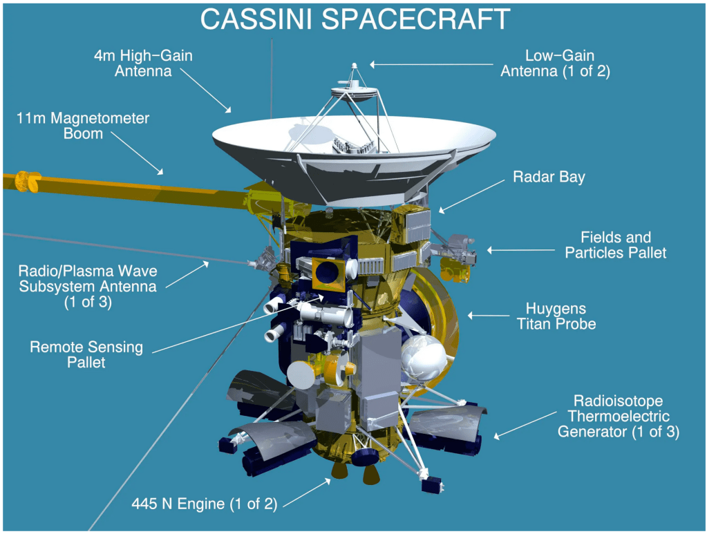
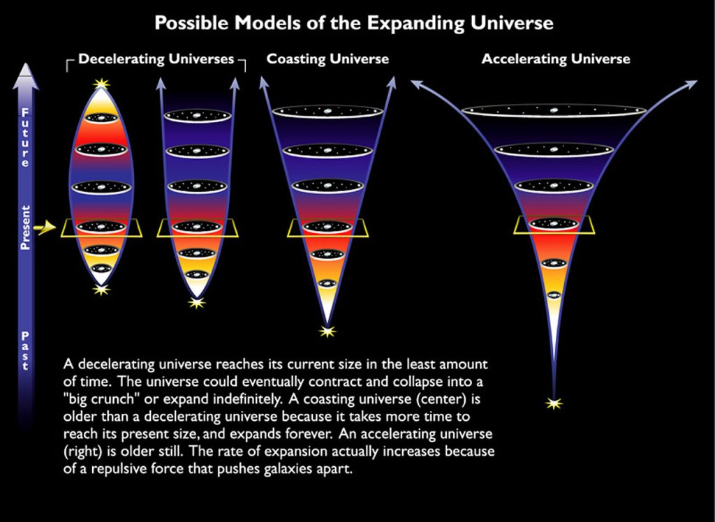
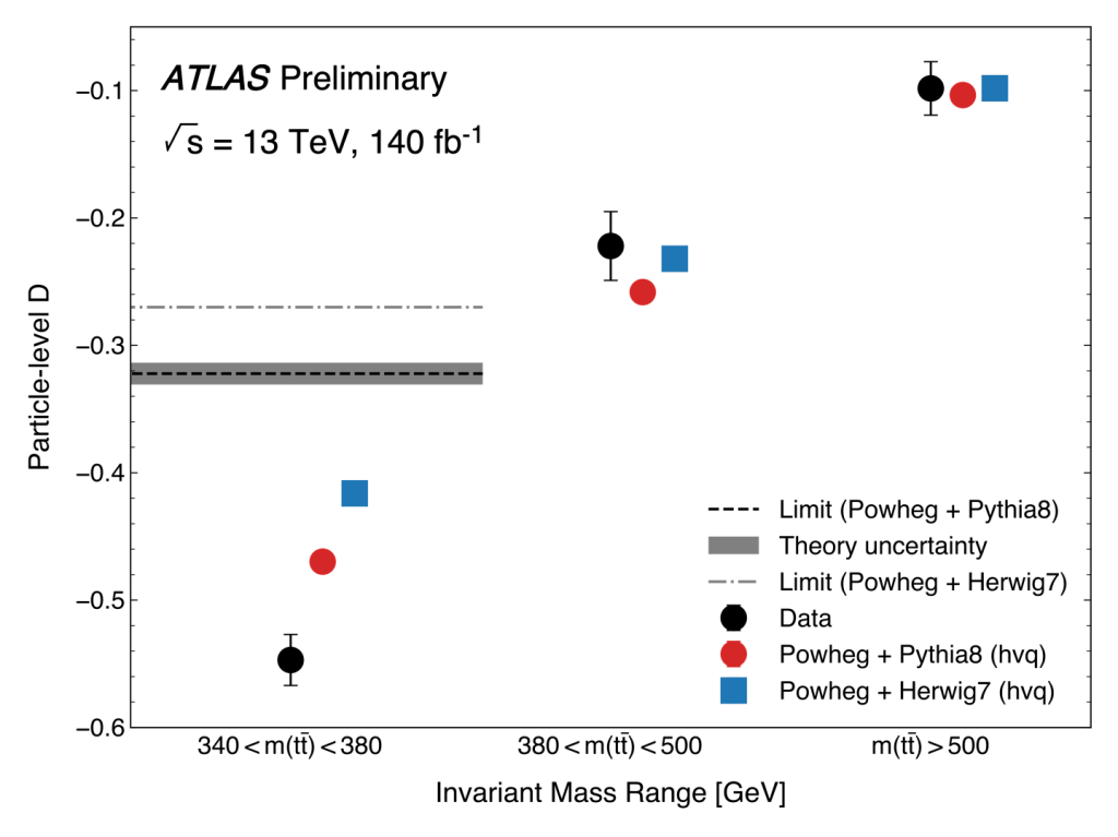


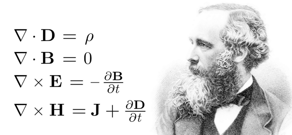
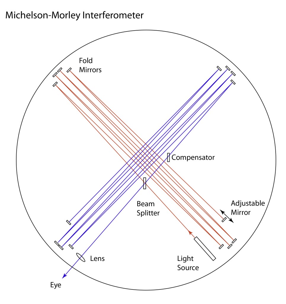
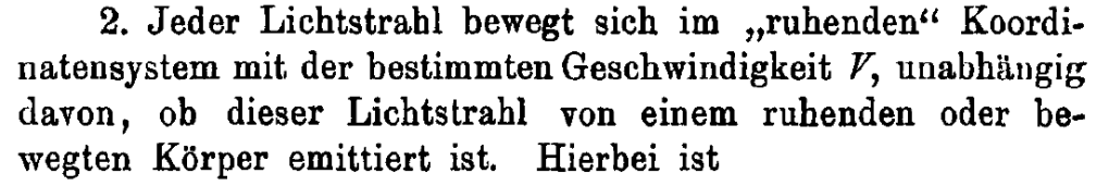
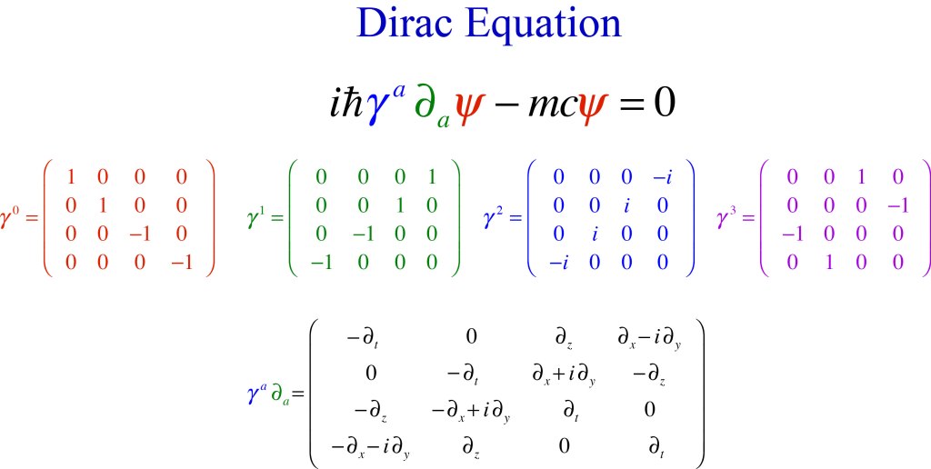
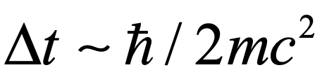
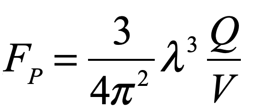
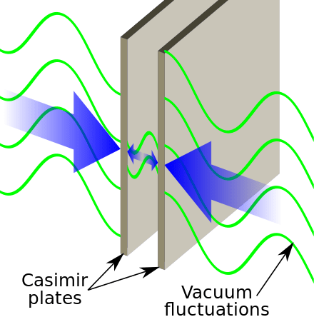


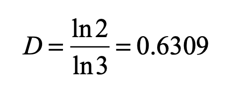
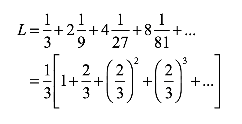
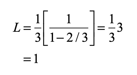


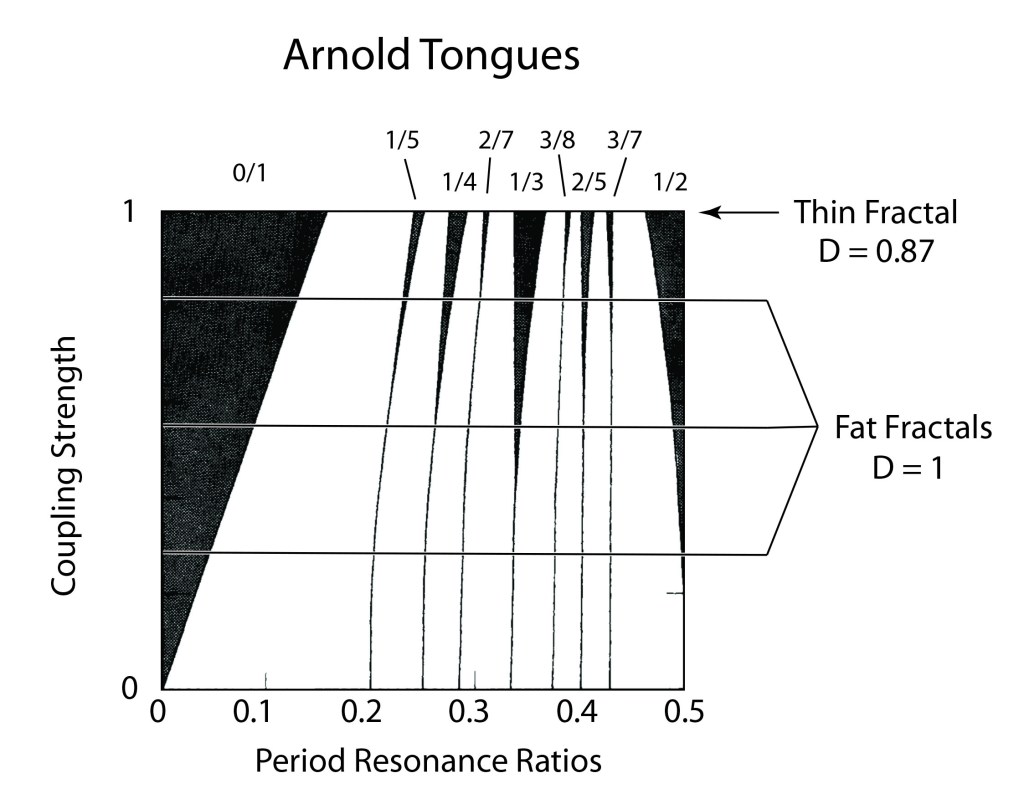

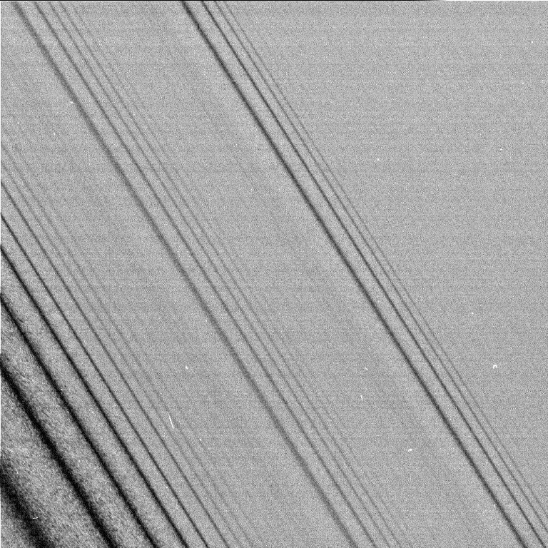
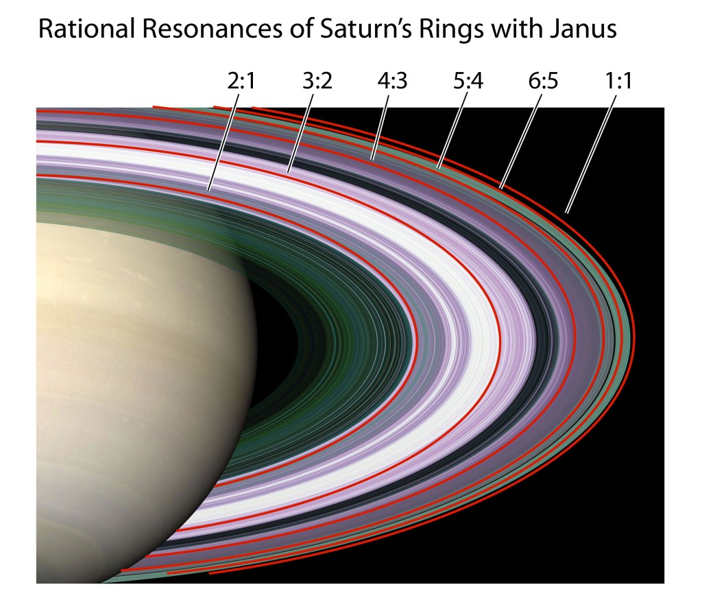


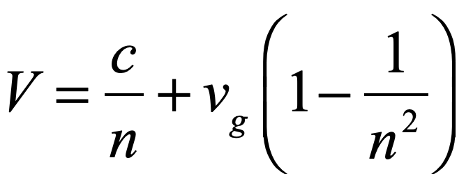
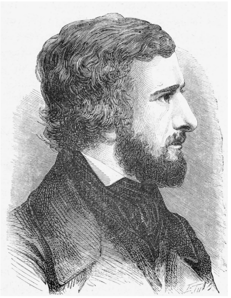
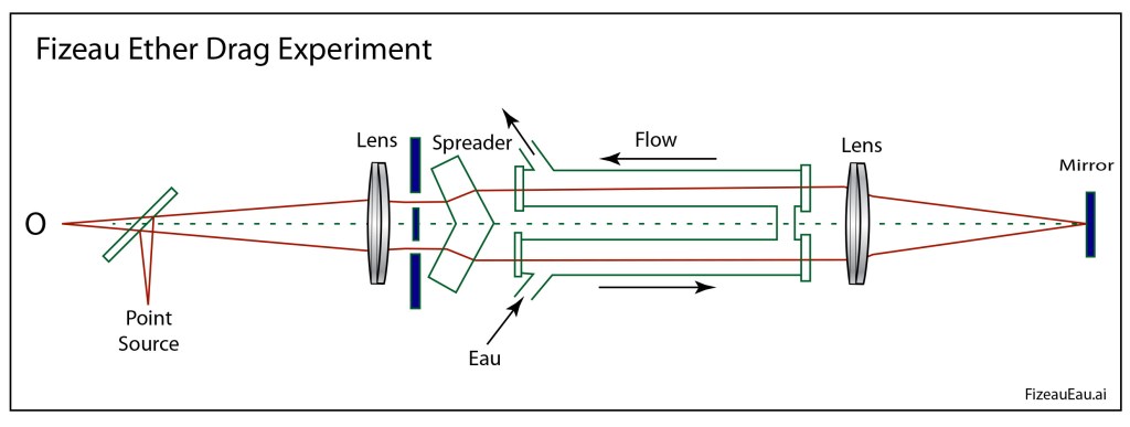
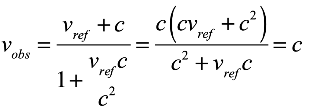
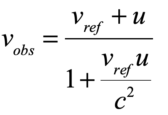


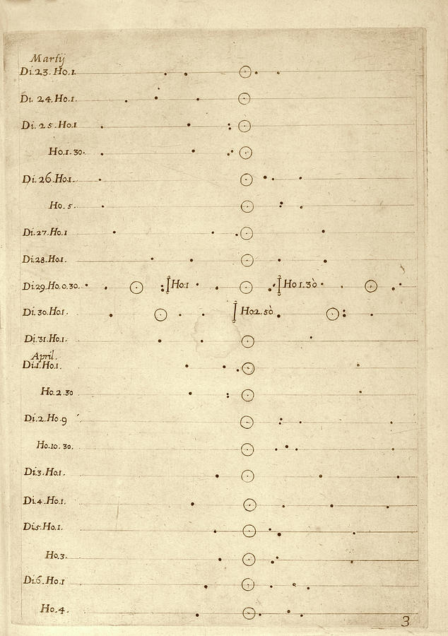

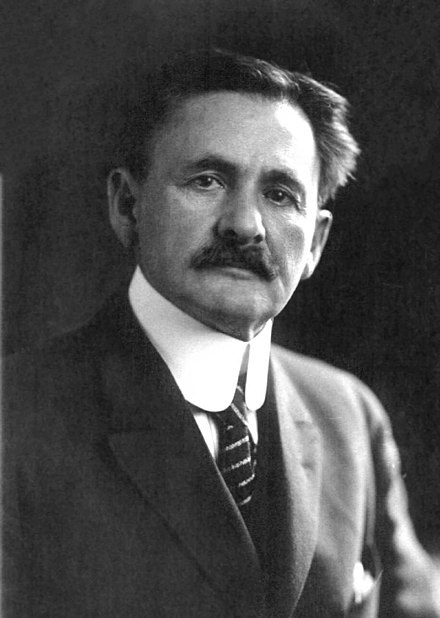

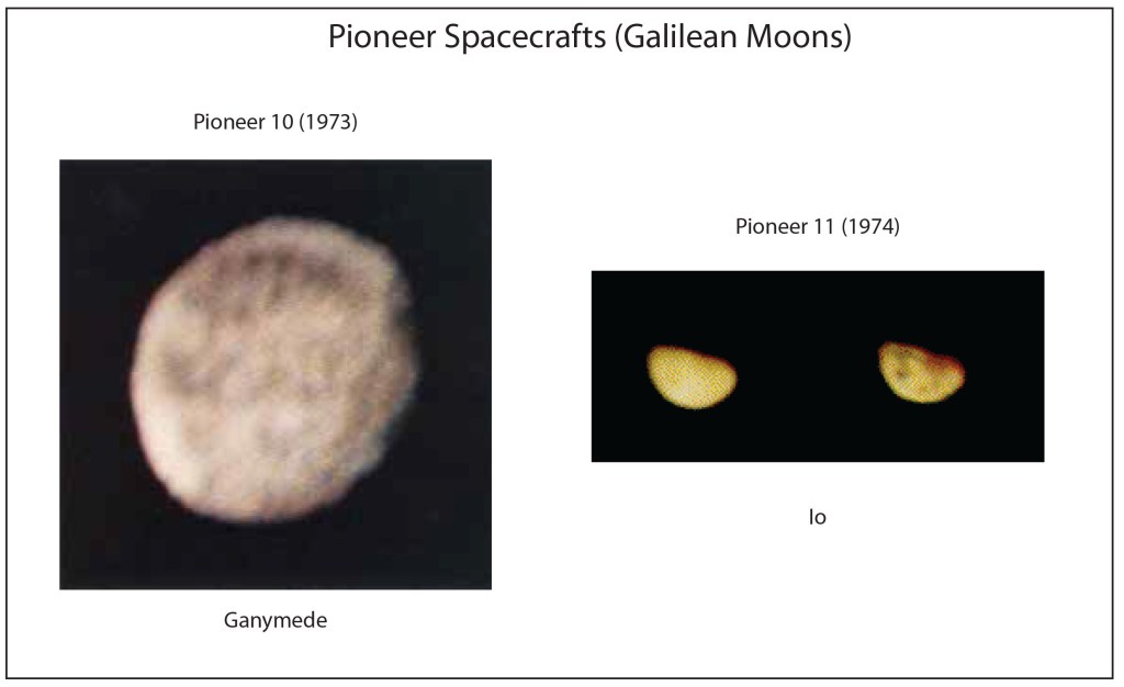


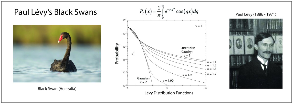


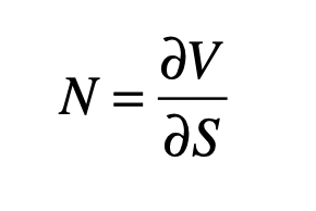
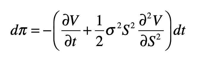
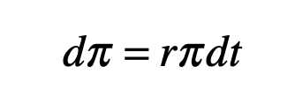
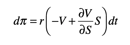
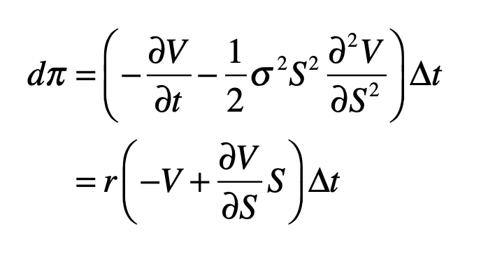
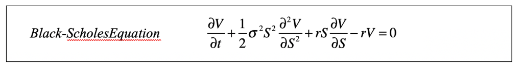
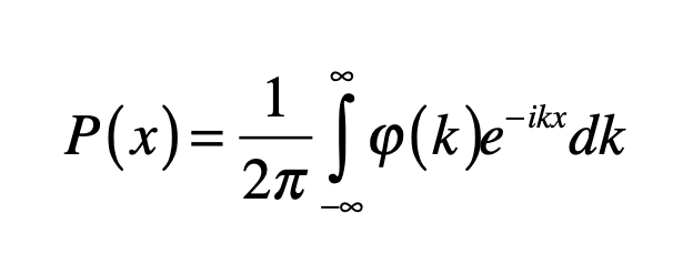
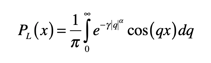

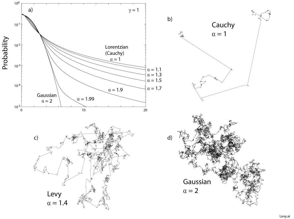


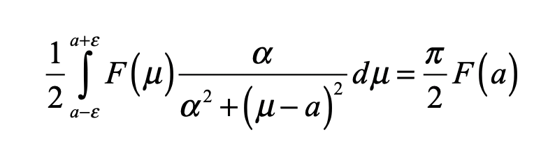
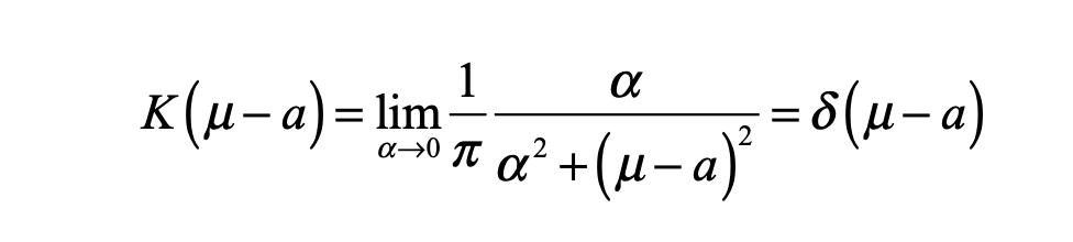

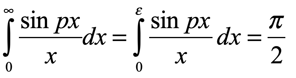
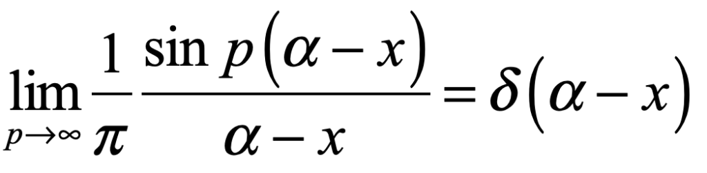


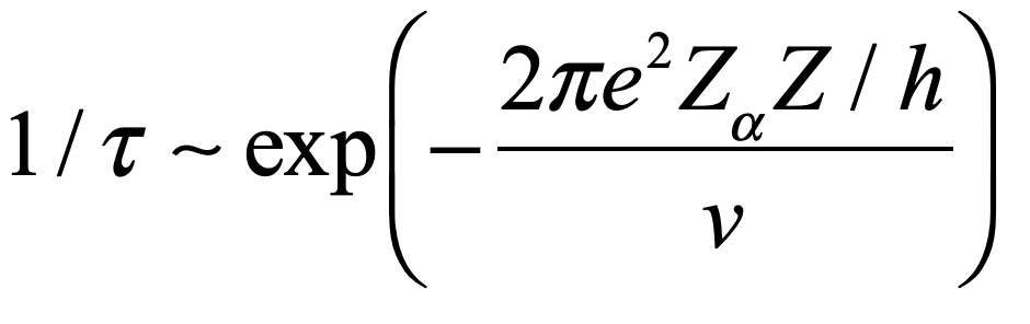
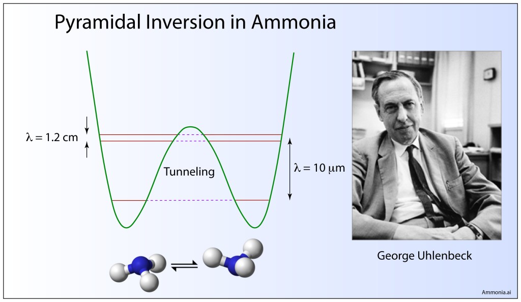
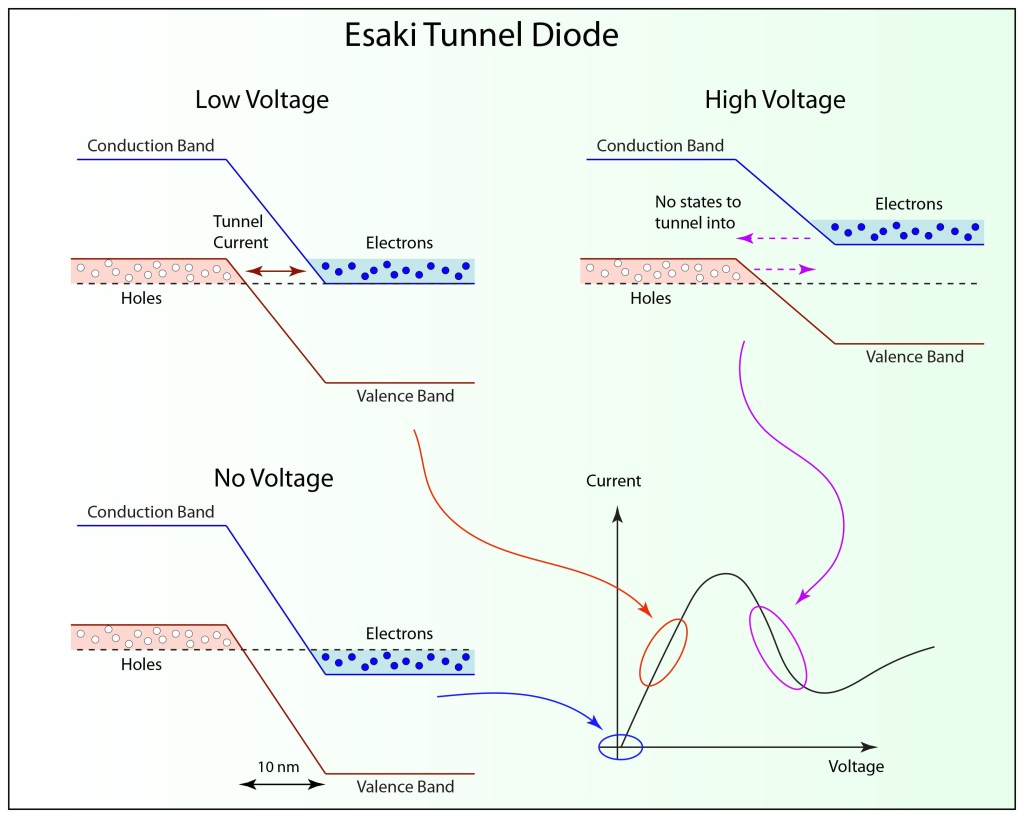
