Hyperspace is neither a fiction nor an abstraction. Every interaction we have with our every-day world occurs in high-dimensional spaces of objects and coordinates and momenta. This dynamical hyperspace—also known as phase space—is as real as mathematics, and physics in phase space can be calculated and used to predict complex behavior. Although phase space can extend to thousands of dimensions, our minds are incapable of thinking even in four dimensions—we have no ability to visualize such things.
Grassmann was convinced that he had discovered a fundamentally new type of mathematics—he actually had.
Part of the trick of doing physics in high dimensions is having the right tools and symbols with which to work. For high-dimensional math and physics, one such indispensable tool is Hermann Grassmann’s wedge product. When I first saw the wedge product, probably in some graduate-level dynamics textbook, it struck me as a little cryptic. It is sort of like a vector product, but not, and it operated on things that had an intimidating name— “forms”. I kept trying to “understand” forms as if they were types of vectors. After all, under special circumstances, forms and wedges did produce some vector identities. It was only after I actually stepped back and asked myself how they were constructed that I realized that forms and wedge products were just a simple form of algebra, called exterior algebra. Exterior algebra is an especially useful form of algebra with simple rules. It goes far beyond vectors while harking back to a time before vectors even existed.
Hermann Grassmann: A Backwater Genius
We are so accustomed to working with oriented objects, like vectors that have a tip and tail, that it is hard to think of a time when that wouldn’t have been natural. Yet in the mid 1800’s, almost no one was thinking of orientations as a part of geometry, and it took real genius to conceive of oriented elements, how to manipulate them, and how to represent them graphically and mathematically. At a time when some of the greatest mathematicians lived—Weierstrass, Möbius, Cauchy, Gauss, Hamilton—it turned out to be a high school teacher from a backwater in Prussia who developed the theory for the first time.
Hermann Grassmann
Hermann Grassmann was the son of a high school teacher at the Gymnasium in Stettin, Prussia, (now Szczecin, Poland) and he inherited his father’s position, but at a lower level. Despite his lack of background and training, he had serious delusions of grandeur, aspiring to teach mathematics at the university in Berlin, even when he was only allowed to teach the younger high school students basic subjects. Nonetheless, Grassmann embarked on a program to educate himself, attending classes at Berlin in mathematics. As part of the requirements to be allowed to teach mathematics to the senior high-school students, he had to submit a thesis on an appropriate topic.
Modern Szczecin.
For years, he had been working on an idea that had originally come from his father about a mathematical theory that could manipulate abstract objects or concepts. He had taken this vague thought and had slowly developed it into a rigorous mathematical form with symbols and manipulations. His mind was one of those that could permute endlessly, and he defined and discovered dozens of different ways that objects could be defined and combined, and he wrote them all down in a tome of excessive size and complexity. When it was time to submit the thesis to the examiners, he had created a broad new system of algebra—at a time when no one recognized what a new algebra even meant, especially not his examiners, who could understand none of it. Fortunately, Grassmann had been corresponding with the famous German mathematician August Möbius over his ideas, and Möbius was encouraging and supportive, and the examiners accepted his thesis and allowed him to teach the upper class-men at his high school.
The Gymnasium in Stettin
Encouraged by his success, Grassmann hoped that Möbius would help him climb even higher to teach in Berlin. Convinced that he had discovered a fundamentally new type of mathematics (he actually had), he decided to publish his thesis as a book under the title Die Lineale Ausdehnungslehre, ein neuer Zweig der Mathematik (The Theory of Linear Extension, a New Branch of Mathematics). He published it out of his own pocket. It is some measure of his delusion that he had thousands printed, but he sold almost none, and piles of the books were stored away to be used later as scrap paper. Möbius likewise distanced himself from Grassmann and his obsessive theories. Discouraged, Grassmann turned his back on mathematics, though he later achieved fame in the field of linguistics. (For more on Grassmann’s ideas and struggle for recognition, see Chapter 4 of Galileo Unbound).
Excerpt from Grassmann’s Ausdehnungslehre (Google Books).
The Odd Identity of Nicholas Bourbaki
If you look up the publication history of the famous French mathematician, Nicholas Bourbaki, you will be amazed to see a publication history that spans from 1935 to 2018 — over 85 years of publications! But if you look in the obituaries, you will see that he died in 1968. It’s pretty impressive to still be publishing 50 years after your death. JRR Tolkein has been doing that regularly, but few others spring to mind.
Actually,
you have been duped! Nicholas is a
fiction, constructed as a hoax by a group of French mathematicians who were
simultaneously deadly serious about the need for a rigorous foundation on which
to educate the new wave of mathematicians in the mid 20th
century. The group was formed during a
mathematics meeting in 1924, organized by André Weil and joined by Henri Cartan
(son of Eli Cartan), Claude Chevalley, Jean Coulomb, Jean Delsarte, Jean
Dieudonné, Charles Ehresmann, René de Possel, and Szolem Mandelbrojt (uncle of
Benoit Mandelbrot). They picked the last
name of a French general, and Weil’s wife named him Nicholas. The group began publishing books under this
pseudonym in 1935 and has continued until the present time. While their publications were entirely
serious, the group from time to time had fun with mild hoaxes, such as posting
his obituary on one occasion and a wedding announcement of his daughter on
another.
The wedge product symbol took several years to mature. Eli Cartan’s book on differential forms published in 1945 used brackets to denote the product instead of the wedge. In Chevally’s book of 1946, he does not use the wedge, but uses a small square, and the book Chevalley wrote in 1951 “Introduction to the Theory of Algebraic Functions of One Variable” still uses a small square. But in 1954, Chevalley uses the wedge symbol in his book on Spinors. He refers to his own book of 1951 (which did not use the wedge) and also to the 1943 version of Bourbaki. The few existing copies of the 1943 Algebra by Bourbaki lie in obscure European libraries. The 1973 edition of the book does indeed use the wedge, although I have yet to get my hands on the original 1943 version. Therefore, the wedge symbol seems to have originated with Chevalley sometime between 1951 and 1954 and gained widespread use after that.
Exterior Algebra
Exterior algebra begins with the definition of an operation on elements. The elements, for example (u, v, w, x, y, z, etc.) are drawn from a vector space in its most abstract form as “tuples”, such that x = [x1, x2, x3, …, xn] in an n-dimensional space. On these elements there is an operation called the “wedge product”, the “exterior product”, or the “Grassmann product”. It is denoted, for example between two elements x and y, as x^y. It captures the sense of orientation through anti-commutativity, such that
As simple as this definition is, it sets up virtually all later manipulations of vectors and their combinations. For instance, we can immediately prove (try it yourself) that the wedge product of a vector element with itself equals zero
Once the elements of the vector space have been defined, it is possible to define “forms” on the vector space. For instance, a 1-form, also known as a vector, is any function
where a, b, c are scalar coefficients. The wedge product of two 1-forms
yields a 2-form, also known as a bivector. This specific example makes a direct connection to the cross product in 3-space as
where the unit vectors are mapped onto the 2-forms
Indeed, many of the vector identities of 3-space can be expressed in terms of exterior products, but these are just special cases, and the wedge product is more general. For instance, while the triple vector cross product is not associative, the wedge product is associative
which can give it an advantage when performing algebra on r-forms. Expressing the wedge product in terms of vector components
yields the immediate generalization to any number of dimensions (using the Einstein summation convention)
In this way, the wedge product expresses relationships in
any number of dimensions.
A 3-form is constructed as the wedge
product of 3 vectors
where the Levi-Civita permuation symbol has been introduced such that
Note that in 3-space there can be no 4-form, because one of the basis elements would be repeated, rendering the product zero. Therefore, the most general multilinear form for 3-space is
with
23 = 8 elements: one scalar, three 1-forms, three 2-forms and one
3-form. In 4-space there are 24
= 16 elements: one scalar, four 1-forms, six 2-forms, four 3-forms and one
4-form. So, the number of elements rises
exponentially with the dimension of the space.
At this point, we have developed a rich multilinear structure, all based on the simple anti-commutativity of elements x^y = -y^x. This process is called by another name: a Clifford algebra, named after William Kingdon Clifford (1845-1879), second wrangler at Cambridge and close friend of Arthur Cayley. But the wedge product is not just algebra—there is also a straightforward geometric interpretation of wedge products that make them useful when extending theories of surfaces and volumes into higher dimensions.
Geometric Interpretation
In Euclidean space, a cross product is related to areas and volumes of paralellapipeds. Wedge products are more general than cross products and they generalize the idea of areas and volumes to higher dimension. As an illustration, an area 2-form is shown in Fig. 1 and a 3-form in Fig. 2.
Fig. 1 Area 2-form showing how the area of a parallelogram is related to the wedge product. The 2-form is an oriented area perpendicular to the unit vector.Fig. 2 A volume 3-form in Euclidean space. The volume of the parallelogram is equal to the magnitude of the wedge product of the three vectors u, v, and w.
The wedge product is not limited to 3 dimensions nor to Euclidean spaces. This is the power and the beauty of Grassmann’s invention. It also generalizes naturally to differential geometry of manifolds producing what are called differential forms. When integrating in higher dimensions or on non-Euclidean manifolds, the most appropriate approach is to use wedge products and differential forms, which will be the topic of my next blog on the generalized Stokes’ theorem.
Further Reading
1. Dieudonné,
J., The Tragedy of Grassmann. Séminaire de Philosophie et Mathématiques 1979,fascicule 2, 1-14.
2. Fearnley-Sander, D., Hermann Grassmann and the Creation of Linear Algegra. American Mathematical Monthly 1979,86 (10), 809-817.
3. Nolte,
D. D., Galileo Unbound: A Path Across Life, the Universe and Everything.
Oxford University Press: 2018.
4. Vargas,
J. G., Differential Geometry for Physicists and Mathematicians: Moving
Frames and Differential Forms: From Euclid Past Riemann. 2014; p 1-293.
The second edition of Introduction to Modern Dynamics: Chaos, Networks, Space and Time is available from Oxford University Press and Amazon.
Most physics majors will use modern dynamics in their careers: nonlinearity, chaos, network theory, econophysics, game theory, neural nets, geodesic geometry, among many others.
The first edition of Introduction to Modern Dynamics (IMD) was an upper-division junior-level mechanics textbook at the level of Thornton and Marion (Classical Dynamics of Particles and Systems) and Taylor (Classical Mechanics). IMD helped lead an emerging trend in physics education to update the undergraduate physics curriculum. Conventional junior-level mechanics courses emphasized Lagrangian and Hamiltonian physics, but notably missing from the classic subjects are modern dynamics topics that most physics majors will use in their careers: nonlinearity, chaos, network theory, econophysics, game theory, neural nets, geodesic geometry, among many others. These are the topics at the forefront of physics that drive high-tech businesses and start-ups, which is where more than half of all physicists work. IMD introduced these modern topics to junior-level physics majors in an accessible form that allowed them to master the fundamentals to prepare them for the modern world.
The second edition (IMD2) continues that trend by expanding the chapters to include additional material and topics. It rearranges several of the introductory chapters for improved logical flow and expands them to include key conventional topics that were missing in the first edition (e.g., Lagrange undetermined multipliers and expanded examples of Lagrangian applications). It is also an opportunity to correct several typographical errors and other errata that students have identified over the past several years. The second edition also has expanded homework problems.
The goal of IMD2 is to strengthen the sections on conventional topics (that students need to master to take their GREs) to make IMD2 attractive as a mainstream physics textbook for broader adoption at the junior level, while continuing the program of updating the topics and approaches that are relevant for the roles that physicists play in the 21st century.
(New Chapters and Sections highlighted in red.)
New Features in Second Edition:
Second Edition Chapters and Sections
Part 1 Geometric Mechanics
• Expanded development of Lagrangian dynamics
• Lagrange multipliers
• More examples of applications
• Connection to statistical mechanics through the virial theorem
• Greater emphasis on action-angle variables
• The key role of adiabatic invariants
Part 1 Geometric Mechanics
Chapter
1 Physics and Geometry
1.1 State space and dynamical flows
1.2 Coordinate representations
1.3 Coordinate transformation
1.4 Uniformly rotating frames
1.5 Rigid-body motion
Chapter
2 Lagrangian Mechanics
2.1 Calculus of variations
2.2 Lagrangian applications
2.3 Lagrange’s undetermined multipliers
2.4 Conservation laws
2.5 Central force motion
2.6 Virial Theorem
Chapter
3 Hamiltonian Dynamics and Phase Space
3.1 The Hamiltonian function
3.2 Phase space
3.3 Integrable systems and action–angle
variables
3.4 Adiabatic invariants
Part 2 Nonlinear Dynamics
• New section on non-autonomous dynamics
• Entire new chapter devoted to Hamiltonian mechanics
• Added importance to Chirikov standard map
• The important KAM theory of “constrained chaos” and solar system stability
• Degeneracy in Hamiltonian chaos
• A short overview of quantum chaos
• Rational resonances and the relation to KAM theory
• A new section of game theory in the context of evolutionary dynamics
• A new section on general equilibrium theory in economics
Part 3 Complex Systems
Chapter
7
Network Dynamics
7.1 Network structures
7.2 Random network topologies
7.3 Synchronization on networks
7.4 Diffusion on networks
7.5 Epidemics on networks
Chapter
8
Evolutionary Dynamics
81 Population dynamics
8.2 Virus infection and immune
deficiency
8.3 Replicator Dynamics
8.4 Quasi-species
8.5 Game theory and evolutionary
stable solutions
Chapter
9
Neurodynamics and Neural Networks
9.1 Neuron structure and function
9.2 Neuron dynamics
9.3 Network nodes: artificial neurons
9.4 Neural network architectures
9.5 Hopfield neural network
9.6 Content-addressable (associative) memory
Chapter
10
Economic Dynamics
10.1 Microeconomics
and equilibrium
10.2 Macroeconomics
10.3
Business cycles
10.4 Random walks and stock prices
(optional)
Part 4 Relativity and Space–Time
• Relativistic trajectories
• Gravitational waves
Part 4 Relativity and Space–Time
Chapter
11
Metric Spaces and Geodesic Motion
11.1 Manifolds and metric tensors
11.2 Derivative of a tensor
11.3 Geodesic curves in configuration
space
11.4 Geodesic motion
Chapter
12
Relativistic Dynamics
12.1 The special theory
12.2 Lorentz transformations
12.3 Metric structure of Minkowski space
12.4 Relativistic trajectories
12.5 Relativistic dynamics
12.6 Linearly accelerating frames
(relativistic)
Chapter
13
The General Theory of Relativity and Gravitation
13.1 Riemann curvature tensor
13.2 The Newtonian correspondence
13.3 Einstein’s field equations
13.4 Schwarzschild space–time
13.5 Kinematic consequences of gravity
13.6 The deflection of light by gravity
13.7 The precession of Mercury’s
perihelion
13.8 Orbits near a black hole
13.9 Gravitational waves
Synopsis of
2nd Ed. Chapters
Chapter 1. Physics
and Geometry (Sample Chapter)
This chapter has been rearranged relative to the 1st edition to provide a more logical flow of the overarching concepts of geometric mechanics that guide the subsequent chapters. The central role of coordinate transformations is strengthened, as is the material on rigid-body motion with expanded examples.
Chapter 2.
Lagrangian Mechanics (Sample Chapter)
Much of the structure and material is retained from the 1st edition while adding two important sections. The section on applications of Lagrangian mechanics adds many direct examples of the use of Lagrange’s equations of motion. An additional new section covers the important topic of Lagrange’s undetermined multipliers
Chapter 3.
Hamiltonian Dynamics and Phase Space (Sample Chapter)
The importance of Hamiltonian systems and dynamics merits a stand-alone chapter. The topics from the 1st edition are expanded in this new chapter, including a new section on adiabatic invariants that plays an important role in the development of quantum theory. Some topics are de-emphasized from the 1st edition, such as general canonical transformations and the symplectic structure of phase space, although the specific transformation to action-angle coordinates is retained and amplified.
Chapter 4. Nonlinear
Dynamics and Chaos
The first part of this chapter is retained from the 1st edition with numerous minor corrections and updates of figures. The second part of the IMD 1st edition, treating Hamiltonian chaos, will be expanded into the new Chapter 5.
Chapter 5.
Hamiltonian Chaos
This new stand-alone chapter expands on the last half of Chapter 3 of the IMD 1st edition. The physical character of Hamiltonian chaos is substantially distinct from dissipative chaos that it deserves its own chapter. It is also a central topic of interest for complex systems that are either conservative or that have integral invariants, such as our N-body solar system that played such an important role in the history of chaos theory beginning with Poincaré. The new chapter highlights Poincaré’s homoclinic tangle, illustrated by the Chirikov Standard Map. The Standard Map is an excellent introduction to KAM theory, which is one of the crowning achievements of the theory of dynamical systems by Komogorov, Arnold and Moser, connecting to deeper aspects of synchronization and rational resonances that drive the structure of systems as diverse as the rotation of the Moon and the rings of Saturn. This is also a perfect lead-in to the next chapter on synchronization. An optional section at the end of this chapter briefly discusses quantum chaos to show how Hamiltonian chaos can be extended into the quantum regime.
Chapter 6.
Synchronization
This is an updated version of the IMD 1st ed. chapter. It has a reduced initial section on coupled linear oscillators, retaining the key ideas about linear eigenmodes but removing some irrelevant details in the 1st edition. A new section is added that defines and emphasizes the importance of quasi-periodicity. A new section on the synchronization of chaotic oscillators is added.
Chapter 7. Network
Dynamics
This chapter rearranges the structure of the chapter from the 1st edition, moving synchronization on networks earlier to connect from the previous chapter. The section on diffusion and epidemics is moved to the back of the chapter and expanded in the 2nd edition into two separate sections on these topics, adding new material on discrete matrix approaches to continuous dynamics.
Chapter 8.
Neurodynamics and Neural Networks
This chapter is retained from the 1st edition with numerous minor corrections and updates of figures.
Chapter 9.
Evolutionary Dynamics
Two new sections are added to this chapter. A section on game theory and evolutionary stable solutions introduces core concepts of evolutionary dynamics that merge well with the other topics of the chapter such as the pay-off matrix and replicator dynamics. A new section on nearly neutral networks introduces new types of behavior that occur in high-dimensional spaces which are counter intuitive but important for understanding evolutionary drift.
Chapter 10. Economic Dynamics
This chapter will be significantly updated relative to the 1st edition. Most of the sections will be rewritten with improved examples and figures. Three new sections will be added. The 1st edition section on consumer market competition will be split into two new sections describing the Cournot duopoly and Pareto optimality in one section, and Walras’ Law and general equilibrium theory in another section. The concept of the Pareto frontier in economics is becoming an important part of biophysical approaches to population dynamics. In addition, new trends in economics are drawing from general equilibrium theory, first introduced by Walras in the nineteenth century, but now merging with modern ideas of fixed points and stable and unstable manifolds. A third new section is added on econophysics, highlighting the distinctions that contrast economic dynamics (phase space dynamical approaches to economics) from the emerging field of econophysics (statistical mechanics approaches to economics).
Chapter 11. Metric
Spaces and Geodesic Motion
This chapter is retained from the 1st edition with several minor corrections and updates of figures.
Chapter 12.
Relativistic Dynamics
This chapter is retained from the 1st edition with minor corrections and updates of figures. More examples will be added, such as invariant mass reconstruction. The connection between relativistic acceleration and Einstein’s equivalence principle will be strengthened.
Chapter 13. The
General Theory of Relativity and Gravitation
This chapter is retained from the 1st edition with minor corrections and updates of figures. A new section will derive the properties of gravitational waves, given the spectacular success of LIGO and the new field of gravitational astronomy.
Homework Problems:
All chapters will have expanded and updated homework problems. Many of the homework problems from the 1st edition will remain, but the number of problems at the end of each chapter will be nearly doubled, while removing some of the less interesting or problematic problems.
It is surprising how much of modern dynamics boils down to an extremely simple formula
This innocuous-looking equation carries such riddles, such surprises, such unintuitive behavior that it can become the object of study for life. This equation is called a vector flow equation, and it can be used to capture the essential physics of economies, neurons, ecosystems, networks, and even orbits of photons around black holes. This equation is to modern dynamics what F = ma was to classical mechanics. It is the starting point for understanding complex systems.
The Magic of Phase Space
The apparent simplicity of the “flow equation” masks the complexity it contains. It is a vector equation because each “dimension” is a variable of a complex system. Many systems of interest may have only a few variables, but ecosystems and economies and social networks may have hundreds or thousands of variables. Expressed in component format, the flow equation is
where the superscript spans the number of variables. But even this masks all that can happen with such an equation. Each of the functions fa can be entirely different from each other, and can be any type of function, whether polynomial, rational, algebraic, transcendental or composite, although they must be single-valued. They are generally nonlinear, and the limitless ways that functions can be nonlinear is where the richness of the flow equation comes from.
The vector flow equation is an ordinary differential equation (ODE) that can be solved for specific trajectories as initial value problems. A single set of initial conditions defines a unique trajectory. For instance, the trajectory for a 4-dimensional example is described as the column vector
which is the single-parameter position vector to a point in phase space, also called state space. The point sweeps through successive configurations as a function of its single parameter—time. This trajectory is also called an orbit. In classical mechanics, the focus has tended to be on the behavior of specific orbits that arise from a specific set of initial conditions. This is the classic “rock thrown from a cliff” problem of introductory physics courses. However, in modern dynamics, the focus shifts away from individual trajectories to encompass the set of all possible trajectories.
Why is Modern Dynamics part of Physics?
If finding the solutions to the “x-dot equals f” vector flow equation is all there is to do, then this would just be a math problem—the solution of ODE’s. There are plenty of gems for mathematicians to look for, and there is an entire of field of study in mathematics called “dynamical systems“, but this would not be “physics”. Physics as a profession is separate and distinct from mathematics, although the two are sometimes confused. Physics uses mathematics as its language and as its toolbox, but physics is not mathematics. Physics is done best when it is done qualitatively—this means with scribbles done on napkins in restaurants or on the back of envelopes while waiting in line. Physics is about recognizing relationships and patterns. Physics is about identifying the limits to scaling properties where the physics changes when scales change. Physics is about the mapping of the simplest possible mathematics onto behavior in the physical world, and recognizing when the simplest possible mathematics is a universal that applies broadly to diverse systems that seem different, but that share the same underlying principles.
So, granted solving ODE’s is not physics, there is still a tremendous amount of good physics that can be done by solving ODE’s. ODE solvers become the modern physicist’s experimental workbench, providing data output from numerical experiments that can test the dependence on parameters in ways that real-world experiments might not be able to access. Physical intuition can be built based on such simulations as the engaged physicist begins to “understand” how the system behaves, able to explain what will happen as the values of parameters are changed.
In the follow sections, three examples of modern dynamics are introduced with a preliminary study, including Python code. These examples are: Galactic dynamics, synchronized networks and ecosystems. Despite their very different natures, their description using dynamical flows share features in common and illustrate the beauty and depth of behavior that can be explored with simple equations.
Galactic Dynamics
One example of the power and beauty of the vector flow equation and its set of all solutions in phase space is called the Henon-Heiles model of the motion of a star within a galaxy. Of course, this is a terribly complicated problem that involves tens of billions of stars, but if you average over the gravitational potential of all the other stars, and throw in a couple of conservation laws, the resulting potential can look surprisingly simple. The motion in the plane of this galactic potential takes two configuration coordinates (x, y) with two associated momenta (px, py) for a total of four dimensions. The flow equations in four-dimensional phase space are simply
Fig. 1 The 4-dimensional phase space flow equations of a star in a galaxy. The terms in light blue are a simple two-dimensional harmonic oscillator. The terms in magenta are the nonlinear contributions from the stars in the galaxy.
where the terms in the light blue box describe a two-dimensional simple harmonic oscillator (SHO), which is a linear oscillator, modified by the terms in the magenta box that represent the nonlinear galactic potential. The orbits of this Hamiltonian system are chaotic, and because there is no dissipation in the model, a single orbit will continue forever within certain ranges of phase space governed by energy conservation, but never quite repeating.
Fig. 2 Two-dimensional Poincaré section of sets of trajectories in four-dimensional phase space for the Henon-Heiles galactic dynamics model. The perturbation parameter is &eps; = 0.3411 and the energy E = 1.
#!/usr/bin/env python3
# -*- coding: utf-8 -*-
"""
Hamilton4D.py
Created on Wed Apr 18 06:03:32 2018

@author: nolte

Derived from:
D. D. Nolte, Introduction to Modern Dynamics: Chaos, Networks, Space and Time, 2nd ed. (Oxford,2019)
"""

import numpy as np
import matplotlib as mpl
from mpl_toolkits.mplot3d import Axes3D
from scipy import integrate
from matplotlib import pyplot as plt
from matplotlib import cm
import time
import os

plt.close('all')

# model_case 1 = Heiles
# model_case 2 = Crescent
print(' ')
print('Hamilton4D.py')
print('Case: 1 = Heiles')
print('Case: 2 = Crescent')
model_case = int(input('Enter the Model Case (1-2)'))

if model_case == 1:
    E = 1       # Heiles: 1, 0.3411   Crescent: 0.05, 1
    epsE = 0.3411   # 3411
    def flow_deriv(x_y_z_w,tspan):
        x, y, z, w = x_y_z_w
        a = z
        b = w
        c = -x - epsE*(2*x*y)
        d = -y - epsE*(x**2 - y**2)
        return[a,b,c,d]
else:
    E = .1       #   Crescent: 0.1, 1
    epsE = 1
    def flow_deriv(x_y_z_w,tspan):
        x, y, z, w = x_y_z_w
        a = z
        b = w
        c = -(epsE*(y-2*x**2)*(-4*x) + x)
        d = -(y-epsE*2*x**2)
        return[a,b,c,d]

prms = np.sqrt(E)
pmax = np.sqrt(2*E)

# Potential Function
if model_case == 1:
    V = np.zeros(shape=(100,100))
    for xloop in range(100):
        x = -2 + 4*xloop/100
        for yloop in range(100):
            y = -2 + 4*yloop/100
            V[yloop,xloop] = 0.5*x**2 + 0.5*y**2 + epsE*(x**2*y - 0.33333*y**3)
else:
    V = np.zeros(shape=(100,100))
    for xloop in range(100):
        x = -2 + 4*xloop/100
        for yloop in range(100):
            y = -2 + 4*yloop/100
            V[yloop,xloop] = 0.5*x**2 + 0.5*y**2 + epsE*(2*x**4 - 2*x**2*y)

fig = plt.figure(1)
contr = plt.contourf(V,100, cmap=cm.coolwarm, vmin = 0, vmax = 10)
fig.colorbar(contr, shrink=0.5, aspect=5)
fig = plt.show()

repnum = 250
mulnum = 64/repnum

np.random.seed(1)
for reploop  in range(repnum):
    px1 = 2*(np.random.random((1))-0.499)*pmax
    py1 = np.sign(np.random.random((1))-0.499)*np.real(np.sqrt(2*(E-px1**2/2)))
    xp1 = 0
    yp1 = 0

    x_y_z_w0 = [xp1, yp1, px1, py1]

    tspan = np.linspace(1,1000,10000)
    x_t = integrate.odeint(flow_deriv, x_y_z_w0, tspan)
    siztmp = np.shape(x_t)
    siz = siztmp[0]

    if reploop % 50 == 0:
        plt.figure(2)
        lines = plt.plot(x_t[:,0],x_t[:,1])
        plt.setp(lines, linewidth=0.5)
        plt.show()
        time.sleep(0.1)
        #os.system("pause")

    y1 = x_t[:,0]
    y2 = x_t[:,1]
    y3 = x_t[:,2]
    y4 = x_t[:,3]

    py = np.zeros(shape=(2*repnum,))
    yvar = np.zeros(shape=(2*repnum,))
    cnt = -1
    last = y1[1]
    for loop in range(2,siz):
        if (last < 0)and(y1[loop] > 0):
            cnt = cnt+1
            del1 = -y1[loop-1]/(y1[loop] - y1[loop-1])
            py[cnt] = y4[loop-1] + del1*(y4[loop]-y4[loop-1])
            yvar[cnt] = y2[loop-1] + del1*(y2[loop]-y2[loop-1])
            last = y1[loop]
        else:
            last = y1[loop]

    plt.figure(3)
    lines = plt.plot(yvar,py,'o',ms=1)
    plt.show()

if model_case == 1:
    plt.savefig('Heiles')
else:
    plt.savefig('Crescent')
Networks, Synchronization and Emergence
A central paradigm of nonlinear science is the emergence of patterns and organized behavior from seemingly random interactions among underlying constituents. Emergent phenomena are among the most awe inspiring topics in science. Crystals are emergent, forming slowly from solutions of reagents. Life is emergent, arising out of the chaotic soup of organic molecules on Earth (or on some distant planet). Intelligence is emergent, and so is consciousness, arising from the interactions among billions of neurons. Ecosystems are emergent, based on competition and symbiosis among species. Economies are emergent, based on the transfer of goods and money spanning scales from the local bodega to the global economy.
One of the common underlying properties of emergence is the existence of networks of interactions. Networks and network science are topics of great current interest driven by the rise of the World Wide Web and social networks. But networks are ubiquitous and have long been the topic of research into complex and nonlinear systems. Networks provide a scaffold for understanding many of the emergent systems. It allows one to think of isolated elements, like molecules or neurons, that interact with many others, like the neighbors in a crystal or distant synaptic connections.
From the point of view of modern dynamics, the state of a node can be a variable or a “dimension” and the interactions among links define the functions of the vector flow equation. Emergence is then something that “emerges” from the dynamical flow as many elements interact through complex networks to produce simple or emergent patterns.
Synchronization is a form of emergence that happens when lots of independent oscillators, each vibrating at their own personal frequency, are coupled together to push and pull on each other, entraining all the individual frequencies into one common global oscillation of the entire system. Synchronization plays an important role in the solar system, explaining why the Moon always shows one face to the Earth, why Saturn’s rings have gaps, and why asteroids are mainly kept away from colliding with the Earth. Synchronization plays an even more important function in biology where it coordinates the beating of the heart and the functioning of the brain.
One of the most dramatic examples of synchronization is the Kuramoto synchronization phase transition. This occurs when a large set of individual oscillators with differing natural frequencies interact with each other through a weak nonlinear coupling. For small coupling, all the individual nodes oscillate at their own frequency. But as the coupling increases, there is a sudden coalescence of all the frequencies into a single common frequency. This mechanical phase transition, called the Kuramoto transition, has many of the properties of a thermodynamic phase transition, including a solution that utilizes mean field theory.
Fig. 3 The Kuramoto model for the nonlinear coupling of N simple phase oscillators. The term in light blue is the simple phase oscillator. The term in magenta is the global nonlinear coupling that connects each oscillator to every other.
The simulation of 20 Poncaré phase oscillators with global coupling is shown in Fig. 4 as a function of increasing coupling coefficient g. The original individual frequencies are spread randomly. The oscillators with similar frequencies are the first to synchronize, forming small clumps that then synchronize with other clumps of oscillators, until all oscillators are entrained to a single compromise frequency. The Kuramoto phase transition is not sharp in this case because the value of N = 20 is too small. If the simulation is run for 200 oscillators, there is a sudden transition from unsynchronized to synchronized oscillation at a threshold value of g.
Fig. 4 The Kuramoto model for 20 Poincare oscillators showing the frequencies as a function of the coupling coefficient.
The Kuramoto phase transition is one of the most important fundamental examples of modern dynamics because it illustrates many facets of nonlinear dynamics in a very simple way. It highlights the importance of nonlinearity, the simplification of phase oscillators, the use of mean field theory, the underlying structure of the network, and the example of a mechanical analog to a thermodynamic phase transition. It also has analytical solutions because of its simplicity, while still capturing the intrinsic complexity of nonlinear systems.
#!/usr/bin/env python3
# -*- coding: utf-8 -*-
"""
Created on Sat May 11 08:56:41 2019

@author: nolte

D. D. Nolte, Introduction to Modern Dynamics: Chaos, Networks, Space and Time, 2nd ed. (Oxford,2019)
"""

# https://www.python-course.eu/networkx.php
# https://networkx.github.io/documentation/stable/tutorial.html
# https://networkx.github.io/documentation/stable/reference/functions.html

import numpy as np
from scipy import integrate
from matplotlib import pyplot as plt
import networkx as nx
from UserFunction import linfit
import time

tstart = time.time()

plt.close('all')

Nfac = 25   # 25
N = 50      # 50
width = 0.2

# model_case 1 = complete graph (Kuramoto transition)
# model_case 2 = Erdos-Renyi
model_case = int(input('Input Model Case (1-2)'))
if model_case == 1:
    facoef = 0.2
    nodecouple = nx.complete_graph(N)
elif model_case == 2:
    facoef = 5
    nodecouple = nx.erdos_renyi_graph(N,0.1)


# function: omegout, yout = coupleN(G)
def coupleN(G):

    # function: yd = flow_deriv(x_y)
    def flow_deriv(y,t0):

        yp = np.zeros(shape=(N,))
        for omloop  in range(N):
            temp = omega[omloop]
            linksz = G.node[omloop]['numlink']
            for cloop in range(linksz):
                cindex = G.node[omloop]['link'][cloop]
                g = G.node[omloop]['coupling'][cloop]

                temp = temp + g*np.sin(y[cindex]-y[omloop])

            yp[omloop] = temp

        yd = np.zeros(shape=(N,))
        for omloop in range(N):
            yd[omloop] = yp[omloop]

        return yd
    # end of function flow_deriv(x_y)

    mnomega = 1.0

    for nodeloop in range(N):
        omega[nodeloop] = G.node[nodeloop]['element']

    x_y_z = omega

    # Settle-down Solve for the trajectories
    tsettle = 100
    t = np.linspace(0, tsettle, tsettle)
    x_t = integrate.odeint(flow_deriv, x_y_z, t)
    x0 = x_t[tsettle-1,0:N]

    t = np.linspace(1,1000,1000)
    y = integrate.odeint(flow_deriv, x0, t)
    siztmp = np.shape(y)
    sy = siztmp[0]

    # Fit the frequency
    m = np.zeros(shape = (N,))
    w = np.zeros(shape = (N,))
    mtmp = np.zeros(shape=(4,))
    btmp = np.zeros(shape=(4,))
    for omloop in range(N):

        if np.remainder(sy,4) == 0:
            mtmp[0],btmp[0] = linfit(t[0:sy//2],y[0:sy//2,omloop]);
            mtmp[1],btmp[1] = linfit(t[sy//2+1:sy],y[sy//2+1:sy,omloop]);
            mtmp[2],btmp[2] = linfit(t[sy//4+1:3*sy//4],y[sy//4+1:3*sy//4,omloop]);
            mtmp[3],btmp[3] = linfit(t,y[:,omloop]);
        else:
            sytmp = 4*np.floor(sy/4);
            mtmp[0],btmp[0] = linfit(t[0:sytmp//2],y[0:sytmp//2,omloop]);
            mtmp[1],btmp[1] = linfit(t[sytmp//2+1:sytmp],y[sytmp//2+1:sytmp,omloop]);
            mtmp[2],btmp[2] = linfit(t[sytmp//4+1:3*sytmp/4],y[sytmp//4+1:3*sytmp//4,omloop]);
            mtmp[3],btmp[3] = linfit(t[0:sytmp],y[0:sytmp,omloop]);


        #m[omloop] = np.median(mtmp)
        m[omloop] = np.mean(mtmp)

        w[omloop] = mnomega + m[omloop]

    omegout = m
    yout = y

    return omegout, yout
    # end of function: omegout, yout = coupleN(G)


Nlink = N*(N-1)//2
omega = np.zeros(shape=(N,))
omegatemp = width*(np.random.rand(N)-1)
meanomega = np.mean(omegatemp)
omega = omegatemp - meanomega
sto = np.std(omega)

lnk = np.zeros(shape = (N,), dtype=int)
for loop in range(N):
    nodecouple.node[loop]['element'] = omega[loop]
    nodecouple.node[loop]['link'] = list(nx.neighbors(nodecouple,loop))
    nodecouple.node[loop]['numlink'] = np.size(list(nx.neighbors(nodecouple,loop)))
    lnk[loop] = np.size(list(nx.neighbors(nodecouple,loop)))

avgdegree = np.mean(lnk)
mnomega = 1

facval = np.zeros(shape = (Nfac,))
yy = np.zeros(shape=(Nfac,N))
xx = np.zeros(shape=(Nfac,))
for facloop in range(Nfac):
    print(facloop)

    fac = facoef*(16*facloop/(Nfac))*(1/(N-1))*sto/mnomega
    for nodeloop in range(N):
        nodecouple.node[nodeloop]['coupling'] = np.zeros(shape=(lnk[nodeloop],))
        for linkloop in range (lnk[nodeloop]):
            nodecouple.node[nodeloop]['coupling'][linkloop] = fac

    facval[facloop] = fac*avgdegree

    omegout, yout = coupleN(nodecouple)                           # Here is the subfunction call for the flow

    for omloop in range(N):
        yy[facloop,omloop] = omegout[omloop]

    xx[facloop] = facval[facloop]

plt.figure(1)
lines = plt.plot(xx,yy)
plt.setp(lines, linewidth=0.5)
plt.show()

elapsed_time = time.time() - tstart
print('elapsed time = ',format(elapsed_time,'.2f'),'secs')
The Web of Life
Ecosystems are among the most complex systems on Earth. The complex interactions among hundreds or thousands of species may lead to steady homeostasis in some cases, to growth and collapse in other cases, and to oscillations or chaos in yet others. But the definition of species can be broad and abstract, referring to businesses and markets in economic ecosystems, or to cliches and acquaintances in social ecosystems, among many other examples. These systems are governed by the laws of evolutionary dynamics that include fitness and survival as well as adaptation.
The dimensionality of the dynamical spaces for these systems extends to hundreds or thousands of dimensions—far too complex to visualize when thinking in four dimensions is already challenging. Yet there are shared principles and common behaviors that emerge even here. Many of these can be illustrated in a simple three-dimensional system that is represented by a triangular simplex that can be easily visualized, and then generalized back to ultra-high dimensions once they are understood.
A simplex is a closed (N-1)-dimensional geometric figure that describes a zero-sum game (game theory is an integral part of evolutionary dynamics) among N competing species. For instance, a two-simplex is a triangle that captures the dynamics among three species. Each vertex of the triangle represents the situation when the entire ecosystem is composed of a single species. Anywhere inside the triangle represents the situation when all three species are present and interacting.
A classic model of interacting species is the replicator equation. It allows for a fitness-based proliferation and for trade-offs among the individual species. The replicator dynamics equations are shown in Fig. 5.
Fig. 5 Replicator dynamics has a surprisingly simple form, but with surprisingly complicated behavior. The key elements are the fitness and the payoff matrix. The fitness relates to how likely the species will survive. The payoff matrix describes how one species gains at the loss of another (although symbiotic relationships also occur).
The population dynamics on the 2D simplex are shown in Fig. 6 for several different pay-off matrices. The matrix values are shown in color and help interpret the trajectories. For instance the simplex on the upper-right shows a fixed point center. This reflects the antisymmetric character of the pay-off matrix around the diagonal. The stable spiral on the lower-left has a nearly asymmetric pay-off matrix, but with unequal off-diagonal magnitudes. The other two cases show central saddle points with stable fixed points on the boundary. A very large variety of behaviors are possible for this very simple system. The Python program is shown in Trirep.py.
Fig. 6 Payoff matrix and population simplex for four random cases: Upper left is an unstable saddle. Upper right is a center. Lower left is a stable spiral. Lower right is a marginal case.
#!/usr/bin/env python3
# -*- coding: utf-8 -*-
"""
trirep.py
Created on Thu May  9 16:23:30 2019

@author: nolte

Derived from:
D. D. Nolte, Introduction to Modern Dynamics: Chaos, Networks, Space and Time, 2nd ed. (Oxford,2019)
"""

import numpy as np
from scipy import integrate
from matplotlib import pyplot as plt

plt.close('all')

def tripartite(x,y,z):

    sm = x + y + z
    xp = x/sm
    yp = y/sm

    f = np.sqrt(3)/2

    y0 = f*xp
    x0 = -0.5*xp - yp + 1;

    plt.figure(2)
    lines = plt.plot(x0,y0)
    plt.setp(lines, linewidth=0.5)
    plt.plot([0, 1],[0, 0],'k',linewidth=1)
    plt.plot([0, 0.5],[0, f],'k',linewidth=1)
    plt.plot([1, 0.5],[0, f],'k',linewidth=1)
    plt.show()


def solve_flow(y,tspan):
    def flow_deriv(y, t0):
    #"""Compute the time-derivative ."""

        f = np.zeros(shape=(N,))
        for iloop in range(N):
            ftemp = 0
            for jloop in range(N):
                ftemp = ftemp + A[iloop,jloop]*y[jloop]
            f[iloop] = ftemp

        phitemp = phi0          # Can adjust this from 0 to 1 to stabilize (but Nth population is no longer independent)
        for loop in range(N):
            phitemp = phitemp + f[loop]*y[loop]
        phi = phitemp

        yd = np.zeros(shape=(N,))
        for loop in range(N-1):
            yd[loop] = y[loop]*(f[loop] - phi);

        if np.abs(phi0) < 0.01:             # average fitness maintained at zero
            yd[N-1] = y[N-1]*(f[N-1]-phi);
        else:                                     # non-zero average fitness
            ydtemp = 0
            for loop in range(N-1):
                ydtemp = ydtemp - yd[loop]
            yd[N-1] = ydtemp

        return yd

    # Solve for the trajectories
    t = np.linspace(0, tspan, 701)
    x_t = integrate.odeint(flow_deriv,y,t)
    return t, x_t

# model_case 1 = zero diagonal
# model_case 2 = zero trace
# model_case 3 = asymmetric (zero trace)
print(' ')
print('trirep.py')
print('Case: 1 = antisymm zero diagonal')
print('Case: 2 = antisymm zero trace')
print('Case: 3 = random')
model_case = int(input('Enter the Model Case (1-3)'))

N = 3
asymm = 3      # 1 = zero diag (replicator eqn)   2 = zero trace (autocatylitic model)  3 = random (but zero trace)
phi0 = 0.001            # average fitness (positive number) damps oscillations
T = 100;


if model_case == 1:
    Atemp = np.zeros(shape=(N,N))
    for yloop in range(N):
        for xloop in range(yloop+1,N):
            Atemp[yloop,xloop] = 2*(0.5 - np.random.random(1))
            Atemp[xloop,yloop] = -Atemp[yloop,xloop]

if model_case == 2:
    Atemp = np.zeros(shape=(N,N))
    for yloop in range(N):
        for xloop in range(yloop+1,N):
            Atemp[yloop,xloop] = 2*(0.5 - np.random.random(1))
            Atemp[xloop,yloop] = -Atemp[yloop,xloop]
        Atemp[yloop,yloop] = 2*(0.5 - np.random.random(1))
    tr = np.trace(Atemp)
    A = Atemp
    for yloop in range(N):
        A[yloop,yloop] = Atemp[yloop,yloop] - tr/N

else:
    Atemp = np.zeros(shape=(N,N))
    for yloop in range(N):
        for xloop in range(N):
            Atemp[yloop,xloop] = 2*(0.5 - np.random.random(1))

    tr = np.trace(Atemp)
    A = Atemp
    for yloop in range(N):
        A[yloop,yloop] = Atemp[yloop,yloop] - tr/N

plt.figure(3)
im = plt.matshow(A,3,cmap=plt.cm.get_cmap('seismic'))  # hsv, seismic, bwr
cbar = im.figure.colorbar(im)

M = 20
delt = 1/M
ep = 0.01;

tempx = np.zeros(shape = (3,))
for xloop in range(M):
    tempx[0] = delt*(xloop)+ep;
    for yloop in range(M-xloop):
        tempx[1] = delt*yloop+ep
        tempx[2] = 1 - tempx[0] - tempx[1]

        x0 = tempx/np.sum(tempx);          # initial populations

        tspan = 70
        t, x_t = solve_flow(x0,tspan)

        y1 = x_t[:,0]
        y2 = x_t[:,1]
        y3 = x_t[:,2]

        plt.figure(1)
        lines = plt.plot(t,y1,t,y2,t,y3)
        plt.setp(lines, linewidth=0.5)
        plt.show()
        plt.ylabel('X Position')
        plt.xlabel('Time')

        tripartite(y1,y2,y3)
Topics in Modern Dynamics
These three examples are just the tip of the iceberg. The topics in modern dynamics are almost numberless. Any system that changes in time is a potential object of study in modern dynamics. Here is a list of a few topics that spring to mind.
The
triumvirate of Cambridge University in the mid-1800’s consisted of three
towering figures of mathematics and physics:
George Stokes (1819 – 1903), William Thomson (1824 – 1907) (Lord
Kelvin), and James Clerk Maxwell (1831 – 1879).
Their discoveries and methodology changed the nature of natural
philosophy, turning it into the subject that today we call physics. Stokes was the elder, establishing himself as
the predominant expert in British mathematical physics, setting the tone for
his close friend Thomson (close in age and temperament) as well as the younger
Maxwell and many other key figures of 19th century British physics.
George Gabriel Stokes was born in County Sligo in Ireland as the youngest son of the rector of Skreen parish of the Church of Ireland. No miraculous stories of his intellectual acumen seem to come from his childhood, as they did for the likes of William Hamilton (1805 – 1865) or George Green (1793 – 1841). Stokes was a good student, attending school in Skreen, then Dublin and Bristol before entering Pembroke College Cambridge in 1837. It was towards the end of his time at Cambridge that he emerged as a top mathematics student and as a candidate for Senior Wrangler.
Church of Ireland church in Skreen, County Sligo, Ireland
The
Cambridge Wrangler
Since 1748, the mathematics course at Cambridge University has held a yearly contest to identify the top graduating mathematics student. The winner of the contest is called the Senior Wrangler, and in the 1800’s the Senior Wrangler received a level of public fame and admiration for intellectual achievement that is somewhat like the fame reserved today for star athletes. In 1824 the mathematics course was reorganized into the Mathematical Tripos, and the contest became known as the Tripos Exam. The depth and length of the exam was legion. For instance, in 1854 when Edward Routh (1831 – 1907) beat out Maxwell for Senior Wrangler, the Tripos consisted of 16 papers spread over 8 days, totaling over 40 hours for a total number of 211 questions. The winner typically scored less than 50%. Famous Senior Wranglers include George Airy, John Herschel, Arthur Cayley, Lord Rayleigh, Arthur Eddington, J. E. Littlewood, Peter Guthrie Tait and Joseph Larmor.
Pembroke College, Cambridge
In his second year at Cambridge, Stokes had begun studying under William Hopkins (1793 – 1866). It was common for mathematics students to have private tutors to prep for the Tripos exam, and Tripos tutors were sometimes as famous as the Senior Wranglers themselves, especially if a tutor (like Hopkins) was to have several students win the exam. George Stokes became Senior Wrangler in 1841, and the same year he won the Smith’s Prize in mathematics. The Tripos tested primarily on bookwork, while the Smith’s Prize tested on originality. To achieve top scores on both designated the student as the most capable and creative mathematician of his class. Stokes was immediately offered a fellowship at Pembroke College allowing him to teach and study whatever he willed.
Part I of the Tripos Exam 1808.
After Stokes graduated, Hopkins
suggested that Stokes study hydrodynamics.
This may have been in part motivated by Hopkins’ own interest is
hydraulic problems in geology, but it was also a prescient suggestion, because
hydrodynamics was poised for a revolution.
The
Early History of Hydrodynamics
Leonardo da Vinci (1452 – 1519) believed that an artist, to capture the essence of a subject, needed to understand its fundamental nature. Therefore, when he was captivated by the idea of portraying the flow of water, he filled his notebooks with charcoal studies of the whorls and vortices of turbulent torrents and waterfalls. He was a budding experimental physicist, recording data on the complex phenomenon of hydrodynamics. Yet Leonardo was no mathematician, and although his understanding of turbulent flow was deep, he did not have the theoretical tools to explain what he saw. Two centuries later, Daniel Bernoulli (1700 – 1782) provided the first mathematical description of water flowing smoothly in his Hydrodynamica (1738). However, the modern language of calculus was only beginning to be used at that time, preventing Daniel from providing a rigorous derivation.
As for nearly all nascent
mathematical theories of the mid 1700’s, whether they be Newtonian dynamics or
the calculus of variations or number and graph theory or population dynamics or
almost anything, the person who placed the theory on firm mathematical
foundations, using modern notions and notations, was Leonhard Euler (1707 –
1783). In 1752 Euler published a treatise
that described the mathematical theory of inviscid flow—meaning flow without
viscosity. Euler’s chief results is
where ρ is the density, v is the velocity, p is pressure, z is the height of the fluid and φ is a velocity potential, while f(t) is a stream function that depends only on time. If the flow is in steady state, the time derivative vanishes, and the stream function is a constant. The key to the inviscid approximation is the dominance of momentum in fast flow, as opposed to creeping flow in which viscosity dominates. Euler’s equation, which expresses the well-known Bernoulli principle, works well under fast laminar conditions, but under slower flow conditions, internal friction ruins the inviscid approximation.
The violation of the inviscid flow
approximation became one of the important outstanding problems in theoretical
physics in the early 1800’s. For
instance, the flow of water around ship’s hulls was a key technological problem
in the strategic need for speed under sail.
In addition, understanding the creation and propagation of water waves
was critical for the safety of ships at sea.
For the growing empire of the British islands, built on the power of
their navy, the physics of hydrodynamics was more than an academic pursuit, and
their archenemy, the French, were leading the way.
The
French Analysts
In
1713 when Newton won his priority dispute with Leibniz over the invention of
calculus, it had the unintended consequence of setting back British mathematics
and physics for over a hundred years. Perhaps
lulled into complacency by their perceived superiority, Cambridge and Oxford
continued teaching classical mathematics, and natural philosophy became
dogmatic as Newton’s in Principia became canon.
Meanwhile Continental mathematical analysis went through a fundamental
transformation. Inspired by Newton’s
Principia rather than revering it, mathematicians such as the Swiss-German
Leonhard Euler, the Frenchwoman Emile du Chatelet and the Italian Joseph
Lagrange pushed mathematical physics far beyond Newton by developing Leibniz’
methods and notations for calculus.
By the early 1800’s, the leading mathematicians of Europe were in the French school led by Pierre-Simon Laplace along with Joseph Fourier, Siméon Denis Poisson and Augustin-Louis Cauchy. In their hands, functional analysis was going through rapid development, both theoretically and applied, far surpassing British mathematics. It was by reading the French analysts in the 1820’s that the Englishman George Green finally helped bring British mathematics back up to speed.
One member of the French school was the French engineer Claude-Louis Navier (1785 – 1836). He was educated at the Ecole Polytechnique and the School for Roads and Bridges where he became one of the leading architects for bridges in France. In addition to his engineering tasks, he also was involved in developing principles of work and kinetic energy that aided the later work of Coriolis, who was one of the first physicists to recognize the explicit interplay between kinetic energy and potential energy. One of Navier’s specialties was hydraulic engineering, and he edited a new edition of a classic work on hydraulics. In the process, he became aware of serious deficiencies in the theoretical treatment of creeping flow, especially with regards to dissipation. By adopting a molecular approach championed by Poisson, including appropriate boundary conditions, he derived a correction to the Euler flow equations that included a new term with a new material property of viscosity
Navier-Stokes Equation
Navier published his new flow equation in 1823, but the publication was followed by years of nasty in-fighting as his assumptions were assaulted by Poisson and others. This acrimony is partly to blame for why Navier was not hailed alone as the discoverer of this equation, which today bears the name “Navier-Stokes Equation”.
Stokes’
Hydrodynamics
Despite the lead of the French mathematicians over the British in mathematical rigor, they were also bogged down by their insistence on mechanistic models that operated on the microscale action-reaction forces. This was true for their theories of elasticity, hydrodynamics as well as the luminiferous ether. George Green in England would change this. While Green was inspired by French mathematics, he made an important shift in thinking in which the fields became the quantities of interest rather than molecular forces. Differential equations describing macroscale phenomena could be “true” independently of any microscale mechanics. His theories on elasticity and light propagation relied on no underlying structure of matter or ether. Underlying models could change, but the differential equations remained true. Maxwell’s equations, a pinnacle of 19th-century British mathematical physics, were field equations that required no microscopic models, although Maxwell and others later tried to devise models of the ether.
George Stokes admired Green and
adopted his mathematics and outlook on natural philosophy. When he turned his attention to hydrodynamic
flow, he adopted a continuum approach that initially did not rely on molecular
interactions to explain viscosity and drag.
He replicated Navier’s results, but this time without relying on any
underlying microscale physics. Yet this
only took him so far. To explain some of
the essential features of fluid pressures he had to revert to microscopic
arguments of isotropy to explain why displacements were linear and why flow at
a boundary ceased. However, once these
functional dependences were set, the remainder of the problem was pure
continuum mechanics, establishing the Navier-Stokes equation for incompressible
flow. Stokes went on to apply no-slip
boundary conditions for fluids flowing through pipes of different geometric
cross sections to calculate flow rates as well as pressure drops along the pipe
caused by viscous drag.
Stokes then turned to experimental results to explain why a pendulum slowly oscillating in air lost amplitude due to dissipation. He reasoned that when the flow of air around the pendulum bob and stiff rod was slow enough the inertial effects would be negligible, simplifying the Navier-Stokes equation. He calculated the drag force on a spherical object moving slowly through a viscous liquid and obtained the now famous law known as Stokes’ Law of Drag
in which the drag force increases linearly with speed and is proportional to viscosity. With dramatic flair, he used his new law to explain why water droplets in clouds float buoyantly until they become big enough to fall as rain.
The
Lucasian Chair of Mathematics
There are rare individuals who become especially respected for the breadth and depth of their knowledge. In our time, already somewhat past, Steven Hawking embodied the ideal of the eminent (almost clairvoyant) scientist pushing his field to the extremes with the deepest understanding, while also being one of the most famous science popularizers of his day as well as an important chronicler of the history of physics. In his own time, Stokes was held in virtually the same level of esteem.
Just as Steven Hawking and Isaac Newton held the Lucasian Chair of Mathematics at Cambridge, Stokes became the Lucasian chair in 1849 and held the chair until his death in 1903. He was offered the chair in part because of the prestige he held as first wrangler and Smith’s prize winner, but also because of his imposing grasp of the central fields of his time. The Lucasian Chair of Mathematics at Cambridge is one of the most famous academic chairs in the world. It was established by Charles II in 1664, and the first Lucasian professor was Isaac Barrow followed by Isaac Newton who held the post for 33 years. Other famous Lucasian professors were Airy, Babbage, Larmor, Dirac as well as Hawking. During his tenure, Stokes made central contributions to hydrodynamics (as we have seen), but also the elasticity of solids, the behavior of waves in elastic solids, the diffraction of light, problems in light, gravity, sound, heat, meteorology, solar physics, and chemistry. Perhaps his most famous contribution was his explanation of fluorescence, for which he won the Rumford Medal. Certainly, if the Nobel Prize had existed in his time, he would have been a Nobel Laureate.
Derivation
of Stokes’ Law
The flow field of an incompressible fluid around a smooth spherical object has zero divergence and satisfies Laplace’s equation. This allows the stream velocities to take the form in spherical coordinates
where the velocity components are defined in terms of the stream function ψ. The partial derivatives of pressure satisfy the equations
where the second-order operator is
The vanishing of the Laplacian of the stream function
allows the function to take the form
The no-slip boundary condition on the surface of the sphere, as well as the asymptotic velocity field far from the sphere taking the form v•cosθ gives the solution
Using this expression in the first equations yields the velocities, pressure and shear
The force on the sphere is obtained by integrating the pressure and the shear stress over the surface of the sphere. The two contributions are
Adding these together gives the final expression for Stokes’ Law
where two thirds of the force is caused by the shear stress and one third by the pressure.
Stokes flow around a sphere. On the left is the pressure. On the right is the y-component of the flow velocity.
Stokes Timeline
1819 – Born County Sligo Parish of Skreen
1837 – Entered Pembroke College Cambridge
1841 – Graduation, Senior Wrangler, Smith’s Prize, Fellow of Pembroke
1845 – Viscosity
1845 – Viscoelastic solid and the luminiferous ether
1845 – Ether drag
1846 – Review of hydrodynamics (including French references)
1847 – Water waves
1847 – Expansion in periodic series (Fourier)
1848 – Jelly theory of the ether
1849 – Lucasian Professorship Cambridge
1849 – Geodesy and Clairaut’s theorem
1849 – Dynamical theory of diffraction
1850 – Damped pendulum, explanation of clouds (water droplets)
1850 – Haidinger’s brushes
1850 – Letter from Kelvin (Thomson) to Stokes on a theorem in vector calculus
1852 – Stokes’ 4 polarization parameters
1852 – Fluorescence and Rumford medal
1854 – Stokes sets “Stokes theorem” for the Smith’s Prize Exam
1857 – Marries
1857 – Effect of wind on sound intensity
1861 – Hankel publishes “Stokes theorem”
1880 – Form of highest waves
1885 – President of Royal Society
1887 – Member of Parliament
1889 – Knighted as baronet by Queen Victoria
1893 – Copley Medal
1903 – Dies
1945 – Cartan establishes modern form of Stokes’ theorem using differential forms
We are exceedingly fortunate that the Earth lies in the Goldilocks zone. This zone is the range of orbital radii of a planet around its sun for which water can exist in a liquid state. Water is the universal solvent, and it may be a prerequisite for the evolution of life. If we were too close to the sun, water would evaporate as steam. And if we are too far, then it would be locked in perpetual ice. As it is, the Earth has had wild swings in its surface temperature. There was once a time, more than 650 million years ago, when the entire Earth’s surface froze over. Fortunately, the liquid oceans remained liquid, and life that already existed on Earth was able to persist long enough to get to the Cambrian explosion. Conversely, Venus may once have had liquid oceans and maybe even nascent life, but too much carbon dioxide turned the planet into an oven and boiled away its water (a fate that may await our own Earth if we aren’t careful). What has saved us so far is the stability of our orbit, our steady distance from the Sun that keeps our water liquid and life flourishing. Yet it did not have to be this way.
The regions of regular motion associated with irrational numbers act as if they were a barrier, restricting the range of chaotic orbits and protecting other nearby orbits from the chaos.
Our solar system is a many-body problem. It consists of three large gravitating bodies (Sun, Jupiter, Saturn) and several minor ones (such as Earth). Jupiter does influence our orbit, and if it were only a few times more massive than it actually is, then our orbit would become chaotic, varying in distance from the sun in unpredictable ways. And if Jupiter were only about 20 times bigger than is actually is, there is a possibility that it would perturb the Earth’s orbit so strongly that it could eject the Earth from the solar system entirely, sending us flying through interstellar space, where we would slowly cool until we became a permanent ice ball. What can protect us from this terrifying fate? What keeps our orbit stable despite the fact that we inhabit a many-body solar system? The answer is number theory!
The Most Irrational Number
What is the most irrational
number you can think of?
Is it: pi = 3.1415926535897932384626433 ?
Or Euler’s constant: e = 2.7182818284590452353602874 ?
How about: sqrt(3) = 1.73205080756887729352744634 ?
These are all perfectly good irrational numbers. But how do you choose the “most irrational” number? The answer is fairly simple. The most irrational number is the one that is least well approximated by a ratio of integers. For instance, it is possible to get close to pi through the ratio 22/7 = 3.1428 which differs from pi by only 4 parts in ten thousand. Or Euler’s constant 87/32 = 2.7188 differs from e by only 2 parts in ten thousand. Yet 87 and 32 are much bigger than 22 and 7, so it may be said that e is more irrational than pi, because it takes ratios of larger integers to get a good approximation. So is there a “most irrational” number? The answer is yes. The Golden Ratio.
The Golden ratio can be defined in many ways, but its most common expression is given by
It is the hardest number to approximate with a ratio of small integers. For instance, to get a number that is as close as one part in ten thousand to the golden mean takes the ratio 89/55. This result may seem obscure, but there is a systematic way to find the ratios of integers that approximate an irrational number. This is known as a convergent from continued fractions.
Continued fractions were invented by John Wallis in 1695, introduced in his book Opera Mathematica. The continued fraction for pi is
An alternate form of displaying this continued fraction is with the expression
The irrational character of pi is captured by the seemingly random integers in this string. However, there can be regular structure in irrational numbers. For instance, a different continued fraction for pi is
that has a surprisingly simple repeating pattern.
The continued fraction for the golden mean has an especially simple repeating form
or
This continued fraction has the slowest convergence for its continued fraction of any other number. Hence, the Golden Ratio can be considered, using this criterion, to be the most irrational number.
If the Golden Ratio is the most irrational number, how does that save us from the chaos of the cosmos? The answer to this question is KAM!
Kolmogorov, Arnold and Moser: (KAM) Theory
KAM is an acronym made from the first initials of three towering mathematicians of the 20th century: Andrey Kolmogorov (1903 – 1987), his student Vladimir Arnold (1937 – 2010), and Jürgen Moser (1928 – 1999).
In 1954, Kolmogorov, considered to be the greatest living mathematician at that time, was invited to give the plenary lecture at a mathematics conference. To the surprise of the conference organizers, he chose to talk on what seemed like a very mundane topic: the question of the stability of the solar system. This had been the topic which Poincaré had attempted to solve in 1890 when he first stumbled on chaotic dynamics. The question had remained open, but the general consensus was that the many-body nature of the solar system made it intrinsically unstable, even for only three bodies.
Against all expectations, Kolmogorov proposed that despite the general chaotic behavior of the three–body problem, there could be “islands of stability” which were protected from chaos, allowing some orbits to remain regular even while other nearby orbits were highly chaotic. He even outlined an approach to a proof of his conjecture, though he had not carried it through to completion.
The proof of Kolmogorov’s conjecture was supplied over the next 10 years through the work of the German mathematician Jürgen Moser and by Kolmogorov’s former student Vladimir Arnold. The proof hinged on the successive ratios of integers that approximate irrational numbers. With this work KAM showed that indeed some orbits are actually protected from neighboring chaos by relying on the irrationality of the ratio of orbital periods.
Resonant Ratios
Let’s go back to the simple model of our solar system that consists of only three bodies: the Sun, Jupiter and Earth. The period of Jupiter’s orbit is 11.86 years, but instead, if it were exactly 12 years, then its period would be in a 12:1 ratio with the Earth’s period. This ratio of integers is called a “resonance”, although in this case it is fairly mismatched. But if this ratio were a ratio of small integers like 5:3, then it means that Jupiter would travel around the sun 5 times in 15 years while the Earth went around 3 times. And every 15 years, the two planets would align. This kind of resonance with ratios of small integers creates a strong gravitational perturbation that alters the orbit of the smaller planet. If the perturbation is strong enough, it could disrupt the Earth’s orbit, creating a chaotic path that might ultimately eject the Earth completely from the solar system.
What KAM discovered is that as the resonance ratio becomes a ratio of large integers, like 87:32, then the planets have a hard time aligning, and the perturbation remains small. A surprising part of this theory is that a nearby orbital ratio might be 5:2 = 1.5, which is only a little different than 87:32 = 1.7. Yet the 5:2 resonance can produce strong chaos, while the 87:32 resonance is almost immune. This way, it is possible to have both chaotic orbits and regular orbits coexisting in the same dynamical system. An irrational orbital ratio protects the regular orbits from chaos. The next question is, how irrational does the orbital ratio need to be to guarantee safety?
You probably already guessed the answer to this question–the answer must be the Golden Ratio. If this is indeed the most irrational number, then it cannot be approximated very well with ratios of small integers, and this is indeed the case. In a three-body system, the most stable orbital ratio would be a ratio of 1.618034. But the more general question of what is “irrational enough” for an orbit to be stable against a given perturbation is much harder to answer. This is the field of Diophantine Analysis, which addresses other questions as well, such as Fermat’s Last Theorem.
KAM Twist Map
The dynamics of three-body systems are hard to visualize directly, so there are tricks that help bring the problem into perspective. The first trick, invented by Henri Poincaré, is called the first return map (or the Poincaré section). This is a way of reducing the dimensionality of the problem by one dimension. But for three bodies, even if they are all in a plane, this still can be complicated. Another trick, called the restricted three-body problem, is to assume that there are two large masses and a third small mass. This way, the dynamics of the two-body system is unaffected by the small mass, so all we need to do is focus on the dynamics of the small body. This brings the dynamics down to two dimensions (the position and momentum of the third body), which is very convenient for visualization, but the dynamics still need solutions to differential equations. So the final trick is to replace the differential equations with simple difference equations that are solved iteratively.
A simple discrete iterative map that captures the essential behavior of the three-body problem begins with action-angle variables that are coupled through a perturbation. Variations on this model have several names: the Twist Map, the Chirikov Map and the Standard Map. The essential mapping is
where J is an action variable (like angular momentum) paired with the angle variable. Initial conditions for the action and the angle are selected, and then all later values are obtained by iteration. The perturbation parameter is given by ε. If ε = 0 then all orbits are perfectly regular and circular. But as the perturbation increases, the open orbits split up into chains of closed (periodic) orbits. As the perturbation increases further, chaotic behavior emerges. The situation for ε = 0.9 is shown in the figure below. There are many regular periodic orbits as well as open orbits. Yet there are simultaneously regions of chaotic behavior. This figure shows an intermediate case where regular orbits can coexist with chaotic ones. The key is the orbital period ratio. For orbital ratios that are sufficiently irrational, the orbits remain open and regular. Bur for orbital ratios that are ratios of small integers, the perturbation is strong enough to drive the dynamics into chaos.
Arnold Twist Map (also known as a Chirikov map) for ε = 0.9 showing the chaos that has emerged at the hyperbolic point, but there are still open orbits that are surprisingly circular (unperturbed) despite the presence of strongly chaotic orbits nearby.
#!/usr/bin/env python3
# -*- coding: utf-8 -*-
"""
Created on Wed Oct. 2, 2019
@author: nolte
"""
import numpy as np
from scipy import integrate
from matplotlib import pyplot as plt
plt.close('all')

eps = 0.9

np.random.seed(2)
plt.figure(1)
for eloop in range(0,50):

    rlast = np.pi*(1.5*np.random.random()-0.5)
    thlast = 2*np.pi*np.random.random()

    orbit = np.int(200*(rlast+np.pi/2))
    rplot = np.zeros(shape=(orbit,))
    thetaplot = np.zeros(shape=(orbit,))
    x = np.zeros(shape=(orbit,))
    y = np.zeros(shape=(orbit,))
    for loop in range(0,orbit):
        rnew = rlast + eps*np.sin(thlast)
        thnew = np.mod(thlast+rnew,2*np.pi)

        rplot[loop] = rnew
        thetaplot[loop] = np.mod(thnew-np.pi,2*np.pi) - np.pi

        rlast = rnew
        thlast = thnew

        x[loop] = (rnew+np.pi+0.25)*np.cos(thnew)
        y[loop] = (rnew+np.pi+0.25)*np.sin(thnew)

    plt.plot(x,y,'o',ms=1)

plt.savefig('StandMapTwist')
The twist map for three values of ε are shown in the figure below. For ε = 0.2, most orbits are open, with one elliptic point and its associated hyperbolic point. At ε = 0.9 the periodic elliptic point is still stable, but the hyperbolic point has generated a region of chaotic orbits. There is still a remnant open orbit that is associated with an orbital period ratio at the Golden Ratio. However, by ε = 0.97, even this most stable orbit has broken up into a chain of closed orbits as the chaotic regions expand.
Twist map for three levels of perturbation.
Safety in Numbers
In our solar system, governed by gravitational attractions, the square of the orbital period increases as the cube of the average radius (Kepler’s third law). Consider the restricted three-body problem of the Sun and Jupiter with the Earth as the third body. If we analyze the stability of the Earth’s orbit as a function of distance from the Sun, the orbital ratio relative to Jupiter would change smoothly. Near our current position, it would be in a 12:1 resonance, but as we moved farther from the Sun, this ratio would decrease. When the orbital period ratio is sufficiently irrational, then the orbit would be immune to Jupiter’s pull. But as the orbital ratio approaches ratios of integers, the effect gets larger. Close enough to Jupiter there would be a succession of radii that had regular motion separated by regions of chaotic motion. The regions of regular motion associated with irrational numbers act as if they were a barrier, restricting the range of chaotic orbits and protecting more distant orbits from the chaos. In this way numbers, rational versus irrational, protect us from the chaos of our own solar system.
A dramatic demonstration of the orbital resonance effect can be seen with the asteroid belt. The many small bodies act as probes of the orbital resonances. The repetitive tug of Jupiter opens gaps in the distribution of asteroid radii, with major gaps, called Kirkwood Gaps, opening at orbital ratios of 3:1, 5:2, 7:3 and 2:1. These gaps are the radii where chaotic behavior occurs, while the regions in between are stable. Most asteroids spend most of their time in the stable regions, because chaotic motion tends to sweep them out of the regions of resonance. This mechanism for the Kirkwood gaps is the same physics that produces gaps in the rings of Saturn at resonances with the many moons of Saturn.
The gaps in the asteroid distributions caused by orbital resonances with Jupiter. Ref. Wikipedia
For a more detailed mathematical description of the KAM theory, see Chapter 5, Hamiltonian Chaos, in Introduction to Modern Dynamics, 2nd edition (Oxford University Press, 2019).
See also:
Dumas, H. S., The KAM Story: A friendly introduction to the content, history and significance of Classical Kolmogorov-Arnold-Moser Theory. World Scientific: 2014.
Arnold, V. I., From superpositions to KAM theory. Vladimir Igorevich Arnold. Selected Papers 1997, PHASIS, 60, 727–740.
The Physics of Life, the Universe and Everything:
Read more about the history of chaos theory in Galileo Unbound from Oxford University Press (2018)
Imagine in your mind the stately grandfather clock. The long slow pendulum swinging back and forth so purposefully with such majesty. It harks back to slower simpler times—seemingly Victorian in character, although their origins go back to Christiaan Huygens in 1656. In introductory physics classes the dynamics of the pendulum is taught as one of the simplest simple harmonic oscillators, only a bit more complicated than a mass on a spring.
But don’t be fooled! This simplicity is an allusion, for the pendulum clock lies at the heart of modern dynamics. It is a nonlinear autonomous oscillator with system gain that balances dissipation to maintain a dynamic equilibrium that ticks on resolutely as long as some energy source can continue to supply it (like the heavy clock weights).
This analysis has converted the two-dimensional dynamics of the autonomous oscillator to a simple one-dimensional dynamics with a stable fixed point.
The dynamic equilibrium of the grandfather clock is known as a limit cycle, and they are the central feature of autonomous oscillators. Autonomous oscillators are one of the building blocks of complex systems, providing the fundamental elements for biological oscillators, neural networks, business cycles, population dynamics, viral epidemics, and even the rings of Saturn. The most famous autonomous oscillator (after the pendulum clock) is named for a Dutch physicist, Balthasar van der Pol (1889 – 1959), who discovered the laws that govern how electrons oscillate in vacuum tubes. But this highly specialized physics problem has expanded to become the new guiding paradigm for the fundamental oscillating element of modern dynamics—the van der Pol oscillator.
The van der Pol Oscillator
The van der Pol (vdP) oscillator begins as a simple harmonic oscillator (SHO) in which the dissipation (loss of energy) is flipped to become gain of energy. This is as simple as flipping the sign of the damping term in the SHO
where β is positive. This 2nd-order ODE is re-written into a dynamical flow as
where γ = β/m is the system gain. Clearly, the dynamics of this SHO with gain would lead to run-away as the oscillator grows without bound.
But no real-world system can grow indefinitely. It has to eventually be limited by things such as inelasticity. One of the simplest ways to include such a limiting process in the mathematical model is to make the gain get smaller at larger amplitudes. This can be accomplished by making the gain a function of the amplitude x as
When the amplitude x gets large, the gain decreases, becoming zero and changing sign when x = 1. Putting this amplitude-dependent gain into the SHO equation yields
This is the van der Pol equation. It is the quintessential example of a nonlinear autonomous oscillator.
When the parameter ε is large, the vdP oscillator has can behave in strongly nonlinear ways, with strongly nonlinear and nonharmonic oscillations. An example is shown in Fig. 2 for a = 5 and b = 2.5. The oscillation is clearly non-harmonic.
Fig. 1 Time trace of the position and velocity of the vdP oscillator with w0 = 5 and ε = 2.5.Fig. 2 State-space portrait of the vdP flow lines for w0 = 5 and ε = 2.5.
#!/usr/bin/env python3
# -*- coding: utf-8 -*-
"""
Created on Mon Apr 16 07:38:57 2018
@author: David Nolte
D. D. Nolte, Introduction to Modern Dynamics: Chaos, Networks, Space and Time, 2nd ed. (Oxford,2019)
"""
import numpy as np
from scipy import integrate
from matplotlib import pyplot as plt

plt.close('all')

def solve_flow(param,lim = [-3,3,-3,3],max_time=10.0):
# van der pol 2D flow
    def flow_deriv(x_y, t0, alpha,beta):
        x, y = x_y
        return [y,-alpha*x+beta*(1-x**2)*y]

    plt.figure()
    xmin = lim[0]
    xmax = lim[1]
    ymin = lim[2]
    ymax = lim[3]
    plt.axis([xmin, xmax, ymin, ymax])

    N=144
    colors = plt.cm.prism(np.linspace(0, 1, N))

    x0 = np.zeros(shape=(N,2))
    ind = -1
    for i in range(0,12):
        for j in range(0,12):
            ind = ind + 1;
            x0[ind,0] = ymin-1 + (ymax-ymin+2)*i/11
            x0[ind,1] = xmin-1 + (xmax-xmin+2)*j/11

    # Solve for the trajectories
    t = np.linspace(0, max_time, int(250*max_time))
    x_t = np.asarray([integrate.odeint(flow_deriv, x0i, t, param)
                      for x0i in x0])

    for i in range(N):
        x, y = x_t[i,:,:].T
        lines = plt.plot(x, y, '-', c=colors[i])
        plt.setp(lines, linewidth=1)

    plt.show()
    plt.title(model_title)
    plt.savefig('Flow2D')

    return t, x_t

def solve_flow2(param,max_time=20.0):
# van der pol 2D flow
    def flow_deriv(x_y, t0, alpha,beta):
        #"""Compute the time-derivative of a Medio system."""
        x, y = x_y
        return [y,-alpha*x+beta*(1-x**2)*y]
    model_title = 'van der Pol Oscillator'
    x0 = np.zeros(shape=(2,))
    x0[0] = 0
    x0[1] = 4.5

    # Solve for the trajectories
    t = np.linspace(0, max_time, int(250*max_time))
    x_t = integrate.odeint(flow_deriv, x0, t, param)

    return t, x_t

param = (5, 2.5)             # van der Pol
lim = (-7,7,-10,10)

t, x_t = solve_flow(param,lim)

t, x_t = solve_flow2(param)
plt.figure(2)
lines = plt.plot(t,x_t[:,0],t,x_t[:,1],'-')
Separation of Time Scales
Nonlinear systems can have very complicated behavior that may be difficult to address analytically. This is why the numerical ODE solver is a central tool of modern dynamics. But there is a very neat analytical trick that can be applied to tame the nonlinearities (if they are not too large) and simplify the autonomous oscillator. This trick is called separation of time scales (also known as secular perturbation theory)—it looks for simultaneous fast and slow behavior within the dynamics. An example of fast and slow time scales in a well-known dynamical system is found in the simple spinning top in which nutation (fast oscillations) are superposed on precession (slow oscillations).
For the autonomous van der Pol oscillator the fast time scale is the natural oscillation frequency, while the slow time scale is the approach to the limit cycle. Let’s assign t0 = t and t1 = εt, where ε is a small parameter. t0 is the slow period (approach to the limit cycle) and t1 is the fast period (natural oscillation frequency). The solution in terms of these time scales is
where x0 is a slow response and acts as an envelope function for x1 that is the fast response. The total differential is
Similarly, to obtain a second derivative
Therefore, the vdP equation in terms of x0 and x1 is
to lowest order. Now separate the orders to zeroth and first orders in ε, respectively,
Solve the first equation (a simple harmonic oscillator)
and plug the solution it into the right-hand side of the second equation to give
The key to secular perturbation theory is to confine dynamics to their own time scales. In other words, the slow dynamics provide the envelope that modulates the fast carrier frequency. The envelope dynamics are contained in the time dependence of the coefficients A and B. Furthermore, the dynamics of x1 should be a homogeneous function of time, which requires each term in the last equation to be zero. Therefore, the dynamical equations for the envelope functions are
These can be transformed into polar coordinates. Because the envelope functions do not depend on the slow time scale, the time derivatives are
With these expressions, the slow dynamics become
where the angular velocity in the fast variable is equal to zero, leaving only the angular velocity of the unperturbed oscillator. (This is analogous to the rotating wave approximation (RWA) in optics, and also equivalent to studying the dynamics in the rotating frame of the unperturbed oscillator.)
Making a final substitution ρ = R/2 gives a very simple set of dynamical equations
These final equations capture the essential properties of the relaxation of the dynamics to the limit cycle. To lowest order (when the gain is weak) the angular frequency is unaffected, and the system oscillates at the natural frequency. The amplitude of the limit cycle equals 1. A deviation in the amplitude from 1 decays slowly back to the limit cycle making it a stable fixed point in the radial dynamics. This analysis has converted the two-dimensional dynamics of the autonomous oscillator to a simple one-dimensional dynamics with a stable fixed point on the radius variable. The phase-space portrait of this simplified autonomous oscillator is shown in Fig. 3. What could be simpler? This simplified autonomous oscillator can be found as a fundamental element of many complex systems.
Fig. 3 The state-space diagram of the simplified autonomous oscillator. Initial conditions relax onto the limit cycle. (Reprinted from Introduction to Modern Dynamics (Oxford, 2019) on pg. 8)
This Blog Post is a Companion to the undergraduate physics textbook Modern Dynamics: Chaos, Networks, Space and Time, 2nd ed. (Oxford, 2019) introducing Lagrangians and Hamiltonians, chaos theory, complex systems, synchronization, neural networks, econophysics and Special and General Relativity.
The
physics of a path of light passing a gravitating body is one of the hardest
concepts to understand in General Relativity, but it is also one of the
easiest. It is hard because there can be
no force of gravity on light even though the path of a photon bends as it
passes a gravitating body. It is easy,
because the photon is following the simplest possible path—a geodesic equation
for force-free motion.
This blog picks up where my last blog left off, having there defined the geodesic equation and presenting the Schwarzschild metric. With those two equations in hand, we could simply solve for the null geodesics (a null geodesic is the path of a light beam through a manifold). But there turns out to be a simpler approach that Einstein came up with himself (he never did like doing things the hard way). He just had to sacrifice the fundamental postulate that he used to explain everything about Special Relativity.
Throwing Special Relativity Under the Bus
The fundamental postulate of Special Relativity states that the speed of light is the same for all observers. Einstein posed this postulate, then used it to derive some of the most astonishing consequences of Special Relativity—like E = mc2. This postulate is at the rock core of his theory of relativity and can be viewed as one of the simplest “truths” of our reality—or at least of our spacetime.
Yet as soon as Einstein began thinking how to extend SR to a more general situation, he realized almost immediately that he would have to throw this postulate out. While the speed of light measured locally is always equal to c, the apparent speed of light observed by a distant observer (far from the gravitating body) is modified by gravitational time dilation and length contraction. This means that the apparent speed of light, as observed at a distance, varies as a function of position. From this simple conclusion Einstein derived a first estimate of the deflection of light by the Sun, though he initially was off by a factor of 2. (The full story of Einstein’s derivation of the deflection of light by the Sun and the confirmation by Eddington is in Chapter 7 of Galileo Unbound (Oxford University Press, 2018).)
The “Optics” of Gravity
The invariant element for a light path moving radially in the Schwarzschild geometry is
The apparent speed of light is
then
where c(r) is always less than c, when observing it from
flat space. The “refractive index” of
space is defined, as for any optical material, as the ratio of the constant speed
divided by the observed speed
Because the Schwarzschild metric has the property
the effective refractive index of warped space-time is
with a divergence at the Schwarzschild
radius.
The refractive index of warped space-time in the limit of weak gravity can be used in the ray equation (also known as the Eikonal equation described in an earlier blog)
where the gradient of the refractive index of space is
The ray equation is then a four-variable flow
These equations represent a 4-dimensional flow for a light ray confined to a plane. The trajectory of any light path is found by using an ODE solver subject to the initial conditions for the direction of the light ray. This is simple for us to do today with Python or Matlab, but it was also that could be done long before the advent of computers by early theorists of relativity like Max von Laue (1879 – 1960).
The Relativity of Max von Laue
In the Fall of 1905 in Berlin, a young German physicist by the name of Max Laue was sitting in the physics colloquium at the University listening to another Max, his doctoral supervisor Max Planck, deliver a seminar on Einstein’s new theory of relativity. Laue was struck by the simplicity of the theory, in this sense “simplistic” and hence hard to believe, but the beauty of the theory stuck with him, and he began to think through the consequences for experiments like the Fizeau experiment on partial ether drag.
Armand Hippolyte Louis Fizeau (1819 – 1896) in 1851 built one of the world’s first optical interferometers and used it to measure the speed of light inside moving fluids. At that time the speed of light was believed to be a property of the luminiferous ether, and there were several opposing theories on how light would travel inside moving matter. One theory would have the ether fully stationary, unaffected by moving matter, and hence the speed of light would be unaffected by motion. An opposite theory would have the ether fully entrained by matter and hence the speed of light in moving matter would be a simple sum of speeds. A middle theory considered that only part of the ether was dragged along with the moving matter. This was Fresnel’s partial ether drag hypothesis that he had arrived at to explain why his friend Francois Arago had not observed any contribution to stellar aberration from the motion of the Earth through the ether. When Fizeau performed his experiment, the results agreed closely with Fresnel’s drag coefficient, which seemed to settle the matter. Yet when Michelson and Morley performed their experiments of 1887, there was no evidence for partial drag.
Even after the exposition by Einstein on relativity in 1905, the disagreement of the Michelson-Morley results with Fizeau’s results was not fully reconciled until Laue showed in 1907 that the velocity addition theorem of relativity gave complete agreement with the Fizeau experiment. The velocity observed in the lab frame is found using the velocity addition theorem of special relativity. For the Fizeau experiment, water with a refractive index of n is moving with a speed v and hence the speed in the lab frame is
The difference in the speed of light between the stationary and the moving water is the difference
where the last term is precisely the Fresnel drag coefficient. This was one of the first definitive “proofs” of the validity of Einstein’s theory of relativity, and it made Laue one of relativity’s staunchest proponents. Spurred on by his success with the Fresnel drag coefficient explanation, Laue wrote the first monograph on relativity theory, publishing it in 1910.
Fig. 1 Front page of von Laue’s textbook, first published in 1910, on Special Relativity (this is a 4-th edition published in 1921).
A Nobel Prize for Crystal X-ray Diffraction
In 1909 Laue became a Privatdozent under Arnold Sommerfeld (1868 – 1951) at the university in Munich. In the Spring of 1912 he was walking in the Englischer Garten on the northern edge of the city talking with Paul Ewald (1888 – 1985) who was finishing his doctorate with Sommerfed studying the structure of crystals. Ewald was considering the interaction of optical wavelength with the periodic lattice when it struck Laue that x-rays would have the kind of short wavelengths that would allow the crystal to act as a diffraction grating to produce multiple diffraction orders. Within a few weeks of that discussion, two of Sommerfeld’s students (Friedrich and Knipping) used an x-ray source and photographic film to look for the predicted diffraction spots from a copper sulfate crystal. When the film was developed, it showed a constellation of dark spots for each of the diffraction orders of the x-rays scattered from the multiple periodicities of the crystal lattice. Two years later, in 1914, Laue was awarded the Nobel prize in physics for the discovery. That same year his father was elevated to the hereditary nobility in the Prussian empire and Max Laue became Max von Laue.
Von Laue was not one to take risks, and he remained conservative in many of his interests. He was immensely respected and played important roles in the administration of German science, but his scientific contributions after receiving the Nobel Prize were only modest. Yet as the Nazis came to power in the early 1930’s, he was one of the few physicists to stand up and resist the Nazi take-over of German physics. He was especially disturbed by the plight of the Jewish physicists. In 1933 he was invited to give the keynote address at the conference of the German Physical Society in Wurzburg where he spoke out against the Nazi rejection of relativity as they branded it “Jewish science”. In his speech he likened Einstein, the target of much of the propaganda, to Galileo. He said, “No matter how great the repression, the representative of science can stand erect in the triumphant certainty that is expressed in the simple phrase: And yet it moves.” Von Laue believed that truth would hold out in the face of the proscription against relativity theory by the Nazi regime. The quote “And yet it moves” is supposed to have been muttered by Galileo just after his abjuration before the Inquisition, referring to the Earth moving around the Sun. Although the quote is famous, it is believed to be a myth.
In an odd side-note of history, von Laue sent his gold Nobel prize medal to Denmark for its safe keeping with Niels Bohr so that it would not be paraded about by the Nazi regime. Yet when the Nazis invaded Denmark, to avoid having the medals fall into the hands of the Nazis, the medal was dissolved in aqua regia by a member of Bohr’s team, George de Hevesy. The gold completely dissolved into an orange liquid that was stored in a beaker high on a shelf through the war. When Denmark was finally freed, the dissolved gold was precipitated out and a new medal was struck by the Nobel committee and re-presented to von Laue in a ceremony in 1951.
The Orbits of Light Rays
Von Laue’s interests always stayed close to the properties of light and electromagnetic radiation ever since he was introduced to the field when he studied with Woldemor Voigt at Göttingen in 1899. This interest included the theory of relativity, and only a few years after Einstein published his theory of General Relativity and Gravitation, von Laue added to his earlier textbook on relativity by writing a second volume on the general theory. The new volume was published in 1920 and included the theory of the deflection of light by gravity.
One of the very few illustrations in his second volume is of light coming into interaction with a super massive gravitational field characterized by a Schwarzschild radius. (No one at the time called it a “black hole”, nor even mentioned Schwarzschild. That terminology came much later.) He shows in the drawing, how light, if incident at just the right impact parameter, would actually loop around the object. This is the first time such a diagram appeared in print, showing the trajectory of light so strongly affected by gravity.
Fig. 2 A page from von Laue’s second volume on relativity (first published in 1920) showing the orbit of a photon around a compact mass with “gravitational cutoff” (later known as a “black hole:”). The figure is drawn semi-quantitatively, but the phenomenon was clearly understood by von Laue.
Python Code: gravlens.py
#!/usr/bin/env python3
# -*- coding: utf-8 -*-
"""
gravlens.py
Created on Tue May 28 11:50:24 2019
@author: nolte
D. D. Nolte, Introduction to Modern Dynamics: Chaos, Networks, Space and Time, 2nd ed. (Oxford,2019)
"""

import numpy as np
import matplotlib as mpl
from mpl_toolkits.mplot3d import Axes3D
from scipy import integrate
from matplotlib import pyplot as plt
from matplotlib import cm
import time
import os

plt.close('all')

def create_circle():
	circle = plt.Circle((0,0), radius= 10, color = 'black')
	return circle

def show_shape(patch):
	ax=plt.gca()
	ax.add_patch(patch)
	plt.axis('scaled')
	plt.show()

def refindex(x,y):

    A = 10
    eps = 1e-6

    rp0 = np.sqrt(x**2 + y**2);

    n = 1/(1 - A/(rp0+eps))
    fac = np.abs((1-9*(A/rp0)**2/8))   # approx correction to Eikonal
    nx = -fac*n**2*A*x/(rp0+eps)**3
    ny = -fac*n**2*A*y/(rp0+eps)**3

    return [n,nx,ny]

def flow_deriv(x_y_z,tspan):
    x, y, z, w = x_y_z

    [n,nx,ny] = refindex(x,y)

    yp = np.zeros(shape=(4,))
    yp[0] = z/n
    yp[1] = w/n
    yp[2] = nx
    yp[3] = ny

    return yp

for loop in range(-5,30):

    xstart = -100
    ystart = -2.245 + 4*loop
    print(ystart)

    [n,nx,ny] = refindex(xstart,ystart)


    y0 = [xstart, ystart, n, 0]

    tspan = np.linspace(1,400,2000)

    y = integrate.odeint(flow_deriv, y0, tspan)

    xx = y[1:2000,0]
    yy = y[1:2000,1]


    plt.figure(1)
    lines = plt.plot(xx,yy)
    plt.setp(lines, linewidth=1)
    plt.show()
    plt.title('Photon Orbits')

c = create_circle()
show_shape(c)
axes = plt.gca()
axes.set_xlim([-100,100])
axes.set_ylim([-100,100])

# Now set up a circular photon orbit
xstart = 0
ystart = 15

[n,nx,ny] = refindex(xstart,ystart)

y0 = [xstart, ystart, n, 0]

tspan = np.linspace(1,94,1000)

y = integrate.odeint(flow_deriv, y0, tspan)

xx = y[1:1000,0]
yy = y[1:1000,1]

plt.figure(1)
lines = plt.plot(xx,yy)
plt.setp(lines, linewidth=2, color = 'black')
plt.show()
One of the most striking effects of gravity on photon trajectories is the possibility for a photon to orbit a black hole in a circular orbit. This is shown in Fig. 3 as the black circular ring for a photon at a radius equal to 1.5 times the Schwarzschild radius. This radius defines what is known as the photon sphere. However, the orbit is not stable. Slight deviations will send the photon spiraling outward or inward.
The Eikonal approximation does not strictly hold under strong gravity, but the Eikonal equations with the effective refractive index of space still yield semi-quantitative behavior. In the Python code, a correction factor is used to match the theory to the circular photon orbits, while still agreeing with trajectories far from the black hole. The results of the calculation are shown in Fig. 3. For large impact parameters, the rays are deflected through a finite angle. At a critical impact parameter, near 3 times the Schwarzschild radius, the ray loops around the black hole. For smaller impact parameters, the rays are captured by the black hole.
Fig. 3 Photon orbits near a black hole calculated using the Eikonal equation and the effective refractive index of warped space. One ray, near the critical impact parameter, loops around the black hole as predicted by von Laue. The central black circle is the black hole with a Schwarzschild radius of 10 units. The black ring is the circular photon orbit at a radius 1.5 times the Schwarzschild radius.
Photons pile up around the black hole at the photon sphere. The first image ever of the photon sphere of a black hole was made earlier this year (announced April 10, 2019). The image shows the shadow of the supermassive black hole in the center of Messier 87 (M87), an elliptical galaxy 55 million light-years from Earth. This black hole is 6.5 billion times the mass of the Sun. Imaging the photosphere required eight ground-based radio telescopes placed around the globe, operating together to form a single telescope with an optical aperture the size of our planet. The resolution of such a large telescope would allow one to image a half-dollar coin on the surface of the Moon, although this telescope operates in the radio frequency range rather than the optical.
Fig. 4 Scientists have obtained the first image of a black hole, using Event Horizon Telescope observations of the center of the galaxy M87. The image shows a bright ring formed as light bends in the intense gravity around a black hole that is 6.5 billion times more massive than the Sun.
Fifty years ago on the 20th of July at nearly 11 o’clock at night, my brothers and I were peering through the screen door of a very small 1960’s Shasta compact car trailer watching the TV set on the picnic table outside the trailer door. Our family was at a camp ground in southern Michigan and the mosquitos were fierce (hence why we were inside the trailer looking out through the screen). Neil Armstrong was about to be the first human to step foot on the Moon. The image on the TV was a fuzzy black and white, with barely recognizable shapes clouded even more by the dirt and dead bugs on the screen, but it is a memory etched in my mind. I was 10 years old and I was convinced that when I grew up I would visit the Moon myself, because by then Moon travel would be like flying to Europe. It didn’t turn out that way, and fifty years later it’s a struggle to even get back there.
The dangers could have become life-threatening for the crew of Apollo 11. If they miscalculated their trajectory home and had bounced off the Earth’s atmosphere, they would have become a tragic demonstration of the chaos of three-body orbits.
So maybe I won’t get to the Moon, but maybe my grandchildren will. And if they do, I hope they know something about the three-body problem in physics, because getting to and from the Moon isn’t as easy as it sounds. Apollo 11 faced real danger at several critical points on its flight plan, but all went perfectly (except overshooting their landing site and that last boulder field right before Armstrong landed). Some of those dangers became life-threatening for the crew of Apollo 13, and if they had miscalculated their trajectory home and had bounced off the Earth’s atmosphere, they would have become a tragic demonstration of the chaos of three-body orbits. In fact, their lifeless spaceship might have returned to the Moon and back to Earth over and over again, caught in an infinite chaotic web.
The complexities of trajectories in the three-body problem arise because there are too few constants of motion and too many degrees of freedom. To get an intuitive picture of how the trajectory behaves, it is best to start with a problem known as the restricted three-body problem.
The Saturn V Booster, perhaps the pinnacle of “muscle and grit” space exploration.
The Restricted Three-Body Problem
The restricted three-body problem was first considered by Leonhard Euler in 1762 (for a further discussion of the history of the three-body problem, see my Blog from July 5). For the special case of circular orbits of constant angular frequency, the motion of the third mass is described by the Lagrangian
where the potential is time dependent because of the motion of the two larger masses. Lagrange approached the problem by adopting a rotating reference frame in which the two larger masses m1 and m2 move along the stationary line defined by their centers. The new angle variable is theta-prime. The Lagrangian in the rotating frame is
where the effective potential is now time independent. The first term in the effective potential is
the Coriolis effect and the second is the centrifugal term. The dynamical flow in the plane is four
dimensional, and the four-dimensional flow is
where the position vectors are in the center-of-mass frame
relative to the positions of the Earth and Moon (x1 and x2) in the rotating frame in which they are at rest along the x-axis.
A single trajectory solved for this flow is shown in Fig. 1 for a tiny object passing back and forth chaotically between the Earth and the Moon. The object is considered to be massless, or at least so small it does not perturb the Earth-Moon system. The energy of the object was selected to allow it to pass over the potential barrier of the Lagrange-Point L1 between the Earth and the Moon. The object spends most of its time around the Earth, but now and then will get into a transfer orbit that brings it around the Moon. This would have been the fate of Apollo 11 if their last thruster burn had failed.
Fig. 1 The trajectory of a tiny object in the planar three-body problem interacting with a large mass (Earth on the left) and a small mass (Moon on the right). The energy of the trajectory allows it to pass back and forth chaotically between proximity to the Earth and proximity to the Moon. The time-duration of the simulation is approximately one decade. The envelope of the trajectories is called the “Hill region” named after one of the the first US astrophysicists George William Hill (1838-1914) who studied the 3-body problem of the Moon.
Contrast the orbit of Fig. 1 with the simple flight plan of Apollo 11 on the banner figure. The chaotic character of the three-body problem emerges for a “random” initial condition. You can play with different initial conditions in the following Python code to explore the properties of this dynamical problem. Note that in this simulation, the mass of the Moon was chosen about 8 times larger than in nature to exaggerate the effect of the Moon.
#!/usr/bin/env python3
# -*- coding: utf-8 -*-
"""
Hill.py
Created on Tue May 28 11:50:24 2019
@author: nolte
D. D. Nolte, Introduction to Modern Dynamics: Chaos, Networks, Space and Time, 2nd ed. (Oxford,2019)
"""

import numpy as np
import matplotlib as mpl
from mpl_toolkits.mplot3d import Axes3D
from scipy import integrate
from matplotlib import pyplot as plt
from matplotlib import cm
import time
import os

plt.close('all')

womega = 1
R = 1
eps = 1e-6

M1 = 1     % Mass of the Earth
M2 = 1/10     % Mass of the Moon
chsi = M2/M1

x1 = -M2*R/(M1+M2)    % Earth location in rotating frame
x2 = x1 + R     % Moon location

def poten(y,c):

    rp0 = np.sqrt(y**2 + c**2);
    thetap0 = np.arctan(y/c);

    rp1 = np.sqrt(x1**2 + rp0**2 - 2*np.abs(rp0*x1)*np.cos(np.pi-thetap0));
    rp2 = np.sqrt(x2**2 + rp0**2 - 2*np.abs(rp0*x2)*np.cos(thetap0));
    V = -M1/rp1 -M2/rp2 - E;

    return [V]

def flow_deriv(x_y_z,tspan):
    x, y, z, w = x_y_z

    r1 = np.sqrt(x1**2 + x**2 - 2*np.abs(x*x1)*np.cos(np.pi-z));
    r2 = np.sqrt(x2**2 + x**2 - 2*np.abs(x*x2)*np.cos(z));

    yp = np.zeros(shape=(4,))
    yp[0] = y
    yp[1] = -womega**2*R**3*(np.abs(x)-np.abs(x1)*np.cos(np.pi-z))/(r1**3+eps) - womega**2*R**3*chsi*(np.abs(x)-abs(x2)*np.cos(z))/(r2**3+eps) + x*(w-womega)**2
    yp[2] = w
    yp[3] = 2*y*(womega-w)/x - womega**2*R**3*chsi*abs(x2)*np.sin(z)/(x*(r2**3+eps)) + womega**2*R**3*np.abs(x1)*np.sin(np.pi-z)/(x*(r1**3+eps))

    return yp

r0 = 0.64   % initial radius
v0 = 0.3    % initial radial speed
theta0 = 0   % initial angle
vrfrac = 1   % fraction of speed in radial versus angular directions

rp1 = np.sqrt(x1**2 + r0**2 - 2*np.abs(r0*x1)*np.cos(np.pi-theta0))
rp2 = np.sqrt(x2**2 + r0**2 - 2*np.abs(r0*x2)*np.cos(theta0))
V = -M1/rp1 - M2/rp2
T = 0.5*v0**2
E = T + V

vr = vrfrac*v0
W = (2*T - v0**2)/r0

y0 = [r0, vr, theta0, W]   % This is where you set the initial conditions

tspan = np.linspace(1,2000,20000)

y = integrate.odeint(flow_deriv, y0, tspan)

xx = y[1:20000,0]*np.cos(y[1:20000,2]);
yy = y[1:20000,0]*np.sin(y[1:20000,2]);

plt.figure(1)
lines = plt.plot(xx,yy)
plt.setp(lines, linewidth=0.5)
plt.show()
In the code, set the position and speed of the Apollo command module on lines 56-59 and put in the initial conditions on line 70. The mass of the Moon in nature is 1/81 of the mass of the Earth, which shrinks the L1 “bottleneck” to a much smaller region that you can explore to see what the fate of the Apollo missions could have been.
As a graduate student in physics at Berkeley in the 1980’s, I took General Relativity (aka GR), from Bruno Zumino, who was a world-famous physicist known as one of the originators of super-symmetry in quantum gravity (not to be confused with super-asymmetry of Cooper-Fowler Big Bang Theory fame). The class textbook was Gravitation and cosmology: principles and applications of the general theory of relativity, by Steven Weinberg, another world-famous physicist, in this case known for grand unification of the electro-weak force with electromagnetism. With so much expertise at hand, how could I fail but to absorb the simple essence of general relativity?
The answer is that I failed miserably. Somehow, I managed to pass the course, but I walked away with nothing! And it bugged me for years. What was so hard about GR? It took me almost a decade teaching undergraduate physics classes at Purdue in the 90’s before I realized that it my biggest obstacle had been language: I kept mistaking the words and terms of GR as if they were English. Words like “general covariance” and “contravariant” and “contraction” and “covariant derivative”. They sounded like English, with lots of “co” prefixes that were hard to keep straight, but they actually are part of a very different language that I call Physics-ese,
Physics-ese is a language that has lots of words that sound like English, and so you think you know what the words mean, but the words have sometimes opposite meanings than what you would guess. And the meanings of Physics-ese are precisely defined, and not something that can be left to interpretation. I learned this while teaching the intro courses to non-majors, because so many times when the students were confused, it turned out that it was because they had mistaken a textbook jargon term to be English. If you told them that the word wasn’t English, but just a token standing for a well-defined object or process, it would unshackle them from their misconceptions.
Then, in the early 00’s when I started to explore the physics of generalized trajectories related to some of my own research interests, I realized that the primary obstacle to my learning anything in the Gravitation course was Physics-ese. So this raised the question in my mind: what would it take to teach GR to undergraduate physics majors in a relatively painless manner? This is my answer.
One of the culprits for my mind block learning GR was
Newton himself. His ubiquitous second
law, taught as F = ma, is surprisingly misleading if one wants to have a more
general understanding of what a trajectory is.
This is particularly the case for light paths, which can be bent by
gravity, yet clearly cannot have any forces acting on them.
The way to fix this is subtle yet simple. First, express Newton’s second law as
which is actually closer to the way that Newton expressed the law in his Principia. In three dimensions for a single particle, these equations represent a 6-dimensional dynamical space called phase space: three coordinate dimensions and three momentum dimensions. Then generalize the vector quantities, like the position vector, to be expressed as xa for the six dynamics variables: x, y, z, px, py, and pz.
Now, as part of Physics-ese, putting the index as a superscript instead as a subscript turns out to be a useful notation when working in higher-dimensional spaces. This superscript is called a “contravariant index” which sounds like English but is uninterpretable without a Physics-ese-to-English dictionary. All “contravariant index” means is “column vector component”. In other words, xa is just the position vector expressed as a column vector
This superscripted index is called a “contravariant” index, but seriously dude, just forget that “contravariant” word from Physics-ese and just think “index”. You already know it’s a column vector.
Then Newton’s second law becomes
where the index a runs from 1 to 6, and the function
Fa is a vector function of the dynamic variables. To spell it out, this is
so it’s a lot easier to write it in the one-line form with
the index notation.
The simple index notation equation is in the standard form for what is called, in Physics-ese, a “mathematical flow”. It is an ODE that can be solved for any set of initial conditions for a given trajectory. Or a whole field of solutions can be considered in a phase-space portrait that looks like the flow lines of hydrodynamics. The phase-space portrait captures the essential physics of the system, whether it is a rock thrown off a cliff, or a photon orbiting a black hole. But to get to that second problem, it is necessary to look deeper into the way that space is described by any set of coordinates, especially if those coordinates are changing from location to location.
What’s so Fictitious about Fictitious Forces?
Freshmen physics students are routinely admonished for talking about “centrifugal” forces (rather than centripetal) when describing circular motion, usually with the statement that centrifugal forces are fictitious—only appearing to be forces when the observer is in the rotating frame. The same is said for the Coriolis force. Yet for being such a “fictitious” force, the Coriolis effect is what drives hurricanes and the colossal devastation they cause. Try telling a hurricane victim that they were wiped out by a fictitious force! Looking closer at the Coriolis force is a good way of understanding how taking derivatives of vectors leads to effects often called “fictitious”, yet it opens the door on some of the simpler techniques in the topic of differential geometry.
To start, consider a vector in a uniformly rotating frame. Such a frame is called “non-inertial” because of the angular acceleration associated with the uniform rotation. For an observer in the rotating frame, vectors are attached to the frame, like pinning them down to the coordinate axes, but the axes themselves are changing in time (when viewed by an external observer in a fixed frame). If the primed frame is the external fixed frame, then a position in the rotating frame is
where R is the position vector of the origin of the rotating frame and r is the position in the rotating frame relative to the origin. The funny notation on the last term is called in Physics-ese a “contraction”, but it is just a simple inner product, or dot product, between the components of the position vector and the basis vectors. A basis vector is like the old-fashioned i, j, k of vector calculus indicating unit basis vectors pointing along the x, y and z axes. The format with one index up and one down in the product means to do a summation. This is known as the Einstein summation convention, so it’s just
Taking the time derivative of the position vector gives
and by the chain rule this must be
where the last term has a time derivative of a basis
vector. This is non-zero because in the
rotating frame the basis vector is changing orientation in time. This term is non-inertial and can be shown
fairly easily (see IMD2 Chapter 1) to be
which is where the centrifugal force comes from. This shows how a so-called fictitious force
arises from a derivative of a basis vector.
The fascinating point of this is that in GR, the force of gravity arises
in almost the same way, making it tempting to call gravity a fictitious force,
despite the fact that it can kill you if you fall out a window. The question is, how does gravity arise from
simple derivatives of basis vectors?
The Geodesic Equation
To teach GR to undergraduates, you cannot expect them to have taken a course in differential geometry, because most of them just don’t have the time in their schedule to take such an advanced mathematics course. In addition, there is far more taught in differential geometry than is needed to make progress in GR. So the simple approach is to teach what they need to understand GR with as little differential geometry as possible, expressed with clear English-to-Physics-ese translations.
For example, consider the partial derivative of a vector expressed in index notation as
Taking the partial derivative, using the always-necessary chain rule, is
where the second term is just like the extra
time-derivative term that showed up in the derivation of the Coriolis
force. The basis vector of a general
coordinate system may change size and orientation as a function of position, so
this derivative is not in general zero.
Because the derivative of a basis vector is so central to the ideas of
GR, they are given their own symbol. It
is
where the new “Gamma” symbol is called a Christoffel symbol. It has lots of indexes, both up and down, which looks daunting, but it can be interpreted as the beta-th derivative of the alpha-th component of the mu-th basis vector. The partial derivative is now
For those of you who noticed that some of the indexes
flipped from alpha to mu and vice versa, you’re right! Swapping repeated indexes in these
“contractions” is allowed and helps make derivations a lot easier, which is
probably why Einstein invented this notation in the first place.
The last step in taking a partial derivative of a vector is to isolate a single vector component Va as
where a new symbol, the del-operator has been
introduced. This del-operator is known
as the “covariant derivative” of the vector component. Again, forget the “covariant” part and just
think “gradient”. Namely, taking the
gradient of a vector in general includes changes in the vector component as
well as changes in the basis vector.
Now that you know how to take the partial derivative of a vector using Christoffel symbols, you are ready to generate the central equation of General Relativity: The geodesic equation.
Everyone knows that a geodesic is the shortest path between two points, like a great circle route on the globe. But it also turns out to be the straightest path, which can be derived using an idea known as “parallel transport”. To start, consider transporting a vector along a curve in a flat metric. The equation describing this process is
Because the Christoffel symbols are zero in a flat space, the covariant derivative and the partial derivative are equal, giving
If the vector is transported parallel to itself, then there is no change in V along the curve, so that
Finally, recognizing
and substituting this in gives
This is the geodesic equation!
Fig. 1 The geodesic equation of motion is for force-free motion through a metric space. The curvature of the trajectory is analogous to acceleration, and the generalized gradient is analogous to a force. The geodesic equation is the “F = ma” of GR.
Putting this in the standard form of a flow gives the geodesic flow equations
The flow defines an ordinary differential equation that
defines a curve that carries its own tangent vector onto itself. The curve is parameterized by a parameter s
that can be identified with path length.
It is the central equation of GR, because it describes how an object
follows a force-free trajectory, like free fall, in any general coordinate
system. It can be applied to simple
problems like the Coriolis effect, or it can be applied to seemingly difficult
problems, like the trajectory of a light path past a black hole.
The Metric Connection
Arriving at the geodesic equation is a major
accomplishment, and you have done it in just a few pages of this blog. But there is still an important missing piece
before we are doing General Relativity of gravitation. We need to connect the Christoffel symbol in
the geodesic equation to the warping of space-time around a gravitating
object.
The warping of space-time by matter and energy is another central piece of GR and is often the central focus of a graduate-level course on the subject. This part of GR does have its challenges leading up to Einstein’s Field Equations that explain how matter makes space bend. But at an undergraduate level, it is sufficient to just describe the bent coordinates as a starting point, then use the geodesic equation to solve for so many of the cool effects of black holes.
So, stating the way that matter bends space-time is as simple as writing down the length element for the Schwarzschild metric of a spherical gravitating mass as
where RS = GM/c2 is the Schwarzschild
radius. (The connection between the
metric tensor gab and the Christoffel symbol can be found in Chapter
11 of IMD2.) It takes only a little work
to find that
This means that if we have the Schwarzschild metric, all we
have to do is take first partial derivatives and we will arrive at the
Christoffel symbols that go into the geodesic equation. Solving for any type of force-free trajectory
is then just a matter of solving ODEs with initial conditions (performed
routinely with numerical ODE solvers in Python, Matlab, Mathematica, etc.).
The first problem we will tackle using the geodesic equation is the deflection of light by gravity. This is the quintessential problem of GR because there cannot be any gravitational force on a photon, yet the path of the photon surely must bend in the presence of gravity. This is possible through the geodesic motion of the photon through warped space time. I’ll take up this problem in my next Blog.
This Blog Post is a Companion to the undergraduate physics textbook Modern Dynamics: Chaos, Networks, Space and Time, 2nd ed. (Oxford, 2019) introducing Lagrangians and Hamiltonians, chaos theory, complex systems, synchronization, neural networks, econophysics and Special and General Relativity.
The 1960’s are known as a time of cultural revolution, but perhaps less known was the revolution that occurred in the science of dynamics. Three towering figures of that revolution were Stephen Smale (1930 – ) at Berkeley, Andrey Kolmogorov (1903 – 1987) in Moscow and his student Vladimir Arnold (1937 – 2010). Arnold was only 20 years old in 1957 when he solved Hilbert’s thirteenth problem (that any continuous function of several variables can be constructed with a finite number of two-variable functions). Only a few years later his work on the problem of small denominators in dynamical systems provided the finishing touches on the long elusive explanation of the stability of the solar system (the problem for which Poincaré won the King Oscar Prize in mathematics in 1889 when he discovered chaotic dynamics ). This theory is known as KAM-theory, using the first initials of the names of Kolmogorov, Arnold and Moser [1]. Building on his breakthrough in celestial mechanics, Arnold’s work through the 1960’s remade the theory of Hamiltonian systems, creating a shift in perspective that has permanently altered how physicists look at dynamical systems.
Hamiltonian Physics on a Torus
Traditionally, Hamiltonian physics is associated with systems of inertial objects that conserve the sum of kinetic and potential energy, in other words, conservative non-dissipative systems. But a modern view (after Arnold) of Hamiltonian systems sees them as hyperdimensional mathematical mappings that conserve volume. The space that these mappings inhabit is phase space, and the conservation of phase-space volume is known as Liouville’s Theorem [2]. The geometry of phase space is called symplectic geometry, and the universal position that symplectic geometry now holds in the physics of Hamiltonian mechanics is largely due to Arnold’s textbook Mathematical Methods of Classical Mechanics (1974, English translation 1978) [3]. Arnold’s famous quote from that text is “Hamiltonian mechanics is geometry in phase space”.
One of the striking aspects of this textbook is the reduction of phase-space geometry to the geometry of a hyperdimensional torus for a large number of Hamiltonian systems. If there are as many conserved quantities as there are degrees of freedom in a Hamiltonian system, then the system is called “integrable” (because you can integrated the equations of motion to find a constant of the motion). Then it is possible to map the physics onto a hyperdimensional torus through the transformation of dynamical coordinates into what are known as “action-angle” coordinates [4]. Each independent angle has an associated action that is conserved during the motion of the system. The periodicity of the dynamical angle coordinate makes it possible to identify it with the angular coordinate of a multi-dimensional torus. Therefore, every integrable Hamiltonian system can be mapped to motion on a multi-dimensional torus (one dimension for each degree of freedom of the system).
Actually, integrable Hamiltonian systems are among the most boring dynamical systems you can imagine. They literally just go in circles (around the torus). But as soon as you add a small perturbation that cannot be integrated they produce some of the most complex and beautiful patterns of all dynamical systems. It was Arnold’s focus on motions on a torus, and perturbations that shift the dynamics off the torus, that led him to propose a simple mapping that captured the essence of Hamiltonian chaos.
The Arnold Cat Map
Motion on a two-dimensional torus is defined by two angles, and trajectories on a two-dimensional torus are simple helixes. If the periodicities of the motion in the two angles have an integer ratio, the helix repeats itself. However, if the ratio of periods (also known as the winding number) is irrational, then the helix never repeats and passes arbitrarily closely to any point on the surface of the torus. This last case leads to an “ergodic” system, which is a term introduced by Boltzmann to describe a physical system whose trajectory fills phase space. The behavior of a helix for rational or irrational winding number is not terribly interesting. It’s just an orbit going in circles like an integrable Hamiltonian system. The helix can never even cross itself.
However, if you could add a new dimension to the torus (or add a new degree of freedom to the dynamical system), then the helix could pass over or under itself by moving into the new dimension. By weaving around itself, a trajectory can become chaotic, and the set of many trajectories can become as mixed up as a bowl of spaghetti. This can be a little hard to visualize, especially in higher dimensions, but Arnold thought of a very simple mathematical mapping that captures the essential motion on a torus, preserving volume as required for a Hamiltonian system, but with the ability for regions to become all mixed up, just like trajectories in a nonintegrable Hamiltonian system.
A unit square is isomorphic to a two-dimensional torus. This means that there is a one-to-one mapping of each point on the unit square to each point on the surface of a torus. Imagine taking a sheet of paper and forming a tube out of it. One of the dimensions of the sheet of paper is now an angle coordinate that is cyclic, going around the circumference of the tube. Now if the sheet of paper is flexible (like it is made of thin rubber) you can bend the tube around and connect the top of the tube with the bottom, like a bicycle inner tube. The other dimension of the sheet of paper is now also an angle coordinate that is cyclic. In this way a flat sheet is converted (with some bending) into a torus.
Arnold’s key idea was to create a transformation that takes the torus into itself, preserving volume, yet including the ability for regions to pass around each other. Arnold accomplished this with the simple map
where the modulus 1 takes the unit square into itself. This transformation can also be expressed as a matrix
followed by taking modulus 1. The transformation matrix is called a Floquet matrix, and the determinant of the matrix is equal to unity, which ensures that volume is conserved.
Arnold decided to illustrate this mapping by using a crude image of the face of a cat (See Fig. 1). Successive applications of the transformation stretch and shear the cat, which is then folded back into the unit square. The stretching and folding preserve the volume, but the image becomes all mixed up, just like mixing in a chaotic Hamiltonian system, or like an immiscible dye in water that is stirred.
Fig. 1 Arnold’s illustration of his cat map from pg. 6 of V. I. Arnold and A. Avez, Ergodic Problems of Classical Mechanics (Benjamin, 1968) [5]
Fig. 2 Arnold Cat Map operation is an iterated succession of stretching with shear of a unit square, and translation back to the unit square. The mapping preserves and mixes areas, and is invertible.
Recurrence
When the transformation matrix is applied to continuous values, it produces a continuous range of transformed values that become thinner and thinner until the unit square is uniformly mixed. However, if the unit square is discrete, made up of pixels, then something very different happens (see Fig. 3). The image of the cat in this case is composed of a 50×50 array of pixels. For early iterations, the image becomes stretched and mixed, but at iteration 50 there are 4 low-resolution upside-down versions of the cat, and at iteration 75 the cat fully reforms, but is upside-down. Continuing on, the cat eventually reappears fully reformed and upright at iteration 150. Therefore, the discrete case displays a recurrence and the mapping is periodic. Calculating the period of the cat map on lattices can lead to interesting patterns, especially if the lattice is composed of prime numbers [6].
Fig. 3 A discrete cat map has a recurrence period. This example with a 50×50 lattice has a period of 150.
The Cat Map and the Golden Mean
The golden mean, or the golden ratio, 1.618033988749895 is never far away when working with Hamiltonian systems. Because the golden mean is the “most irrational” of all irrational numbers, it plays an essential role in KAM theory on the stability of the solar system. In the case of Arnold’s cat map, it pops up its head in several ways. For instance, the transformation matrix has eigenvalues
with the remarkable property that
which guarantees conservation of area.
Selected V. I. Arnold Publications
Arnold,
V. I. “FUNCTIONS OF 3 VARIABLES.” Doklady Akademii Nauk Sssr 114(4):
679-681. (1957)
Arnold,
V. I. “GENERATION OF QUASI-PERIODIC MOTION FROM A FAMILY OF PERIODIC
MOTIONS.” Doklady Akademii Nauk Sssr 138(1): 13-&.
(1961)
Arnold,
V. I. “STABILITY OF EQUILIBRIUM POSITION OF A HAMILTONIAN SYSTEM OF
ORDINARY DIFFERENTIAL EQUATIONS IN GENERAL ELLIPTIC CASE.” Doklady
Akademii Nauk Sssr 137(2): 255-&. (1961)
Arnold,
V. I. “BEHAVIOUR OF AN ADIABATIC INVARIANT WHEN HAMILTONS FUNCTION IS
UNDERGOING A SLOW PERIODIC VARIATION.” Doklady Akademii Nauk Sssr 142(4):
758-&. (1962)
Arnold,
V. I. “CLASSICAL THEORY OF PERTURBATIONS AND PROBLEM OF STABILITY OF
PLANETARY SYSTEMS.” Doklady Akademii Nauk Sssr 145(3):
487-&. (1962)
Arnold,
V. I. “BEHAVIOUR OF AN ADIABATIC INVARIANT WHEN HAMILTONS FUNCTION IS
UNDERGOING A SLOW PERIODIC VARIATION.” Doklady Akademii Nauk Sssr 142(4):
758-&. (1962)
Arnold,
V. I. and Y. G. Sinai. “SMALL PERTURBATIONS OF AUTHOMORPHISMS OF A
TORE.” Doklady Akademii Nauk Sssr 144(4): 695-&. (1962)
Arnold,
V. I. “Small denominators and problems of the stability of motion in
classical and celestial mechanics (in Russian).” Usp. Mat. Nauk. 18:
91-192. (1963)
Arnold,
V. I. and A. L. Krylov. “UNIFORM DISTRIBUTION OF POINTS ON A SPHERE AND
SOME ERGODIC PROPERTIES OF SOLUTIONS TO LINEAR ORDINARY DIFFERENTIAL EQUATIONS
IN COMPLEX REGION.” Doklady Akademii Nauk Sssr 148(1):
9-&. (1963)
Arnold,
V. I. “INSTABILITY OF DYNAMICAL SYSTEMS WITH MANY DEGREES OF
FREEDOM.” Doklady Akademii Nauk Sssr 156(1): 9-&. (1964)
Arnold,
V. “SUR UNE PROPRIETE TOPOLOGIQUE DES APPLICATIONS GLOBALEMENT CANONIQUES
DE LA MECANIQUE CLASSIQUE.” Comptes Rendus Hebdomadaires Des Seances De
L Academie Des Sciences 261(19): 3719-&. (1965)
Arnold, V. I. “APPLICABILITY CONDITIONS AND ERROR ESTIMATION BY AVERAGING FOR SYSTEMS WHICH GO THROUGH RESONANCES IN COURSE OF EVOLUTION.” Doklady Akademii Nauk Sssr 161(1): 9-&. (1965)
Bibliography
[1] Dumas, H. S. The KAM Story: A friendly introduction to the content, history and significance of Classical Kolmogorov-Arnold-Moser Theory, World Scientific. (2014)
[2] See Chapter 6, “The Tangled Tale of Phase Space” in Galileo Unbound (D. D. Nolte, Oxford University Press, 2018)
[3] V. I. Arnold, Mathematical Methods of Classical Mechanics (Nauk 1974, English translation Springer 1978)
[4] See Chapter 3, “Hamiltonian Dynamics and Phase Space” in Introduction to Modern Dynamics, 2nd ed. (D. D. Nolte, Oxford University Press, 2019)
[5] V. I. Arnold and A. Avez, Ergodic Problems of Classical Mechanics (Benjamin, 1968)
[6] Gaspari, G. “THE ARNOLD CAT MAP ON PRIME LATTICES.” Physica D-Nonlinear Phenomena 73(4): 352-372. (1994)
This Blog Post is a Companion to the undergraduate physics textbook Modern Dynamics: Chaos, Networks, Space and Time, 2nd ed. (Oxford, 2019) introducing Lagrangians and Hamiltonians, chaos theory, complex systems, synchronization, neural networks, econophysics and Special and General Relativity.


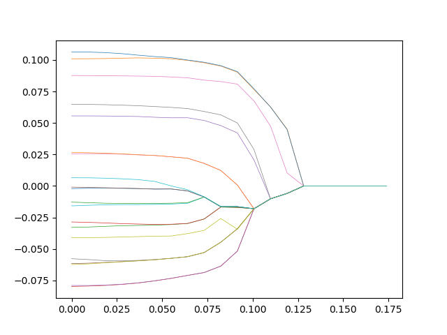


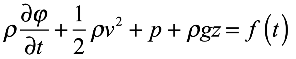
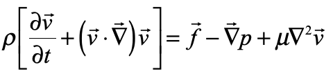
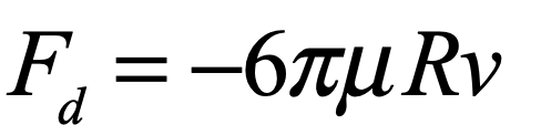
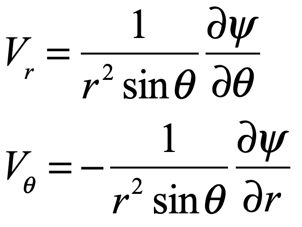
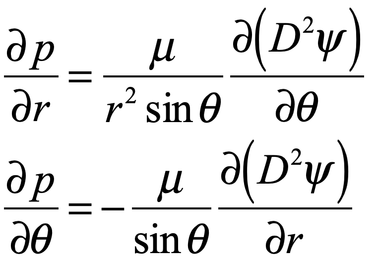
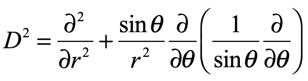

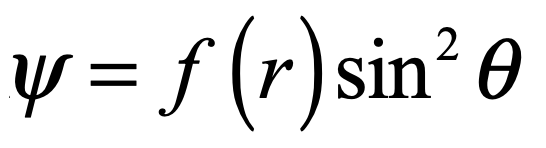
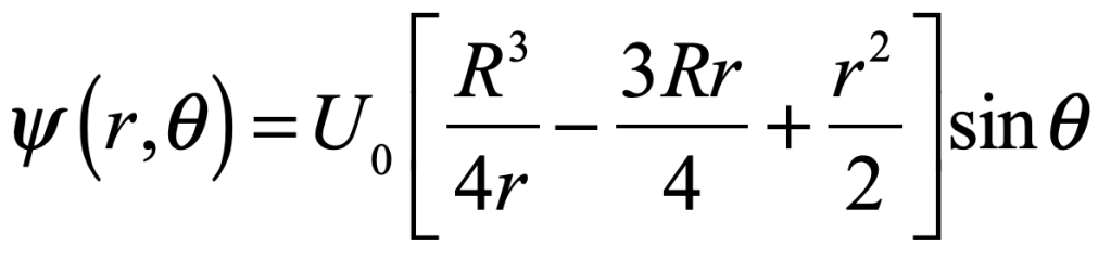
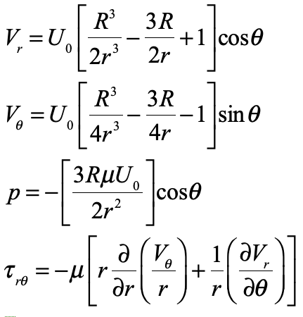
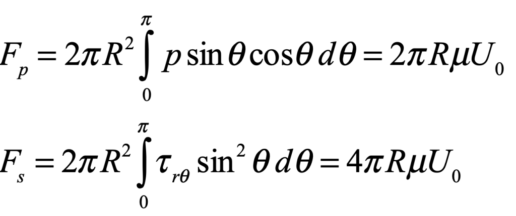
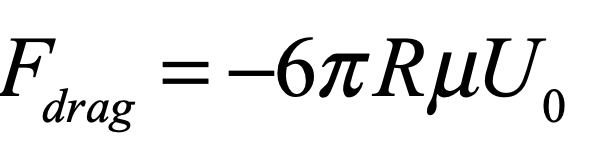
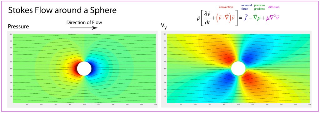

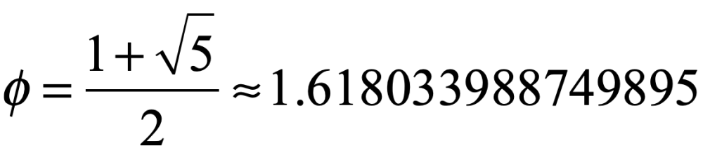
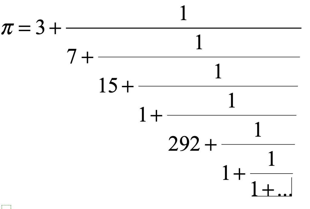


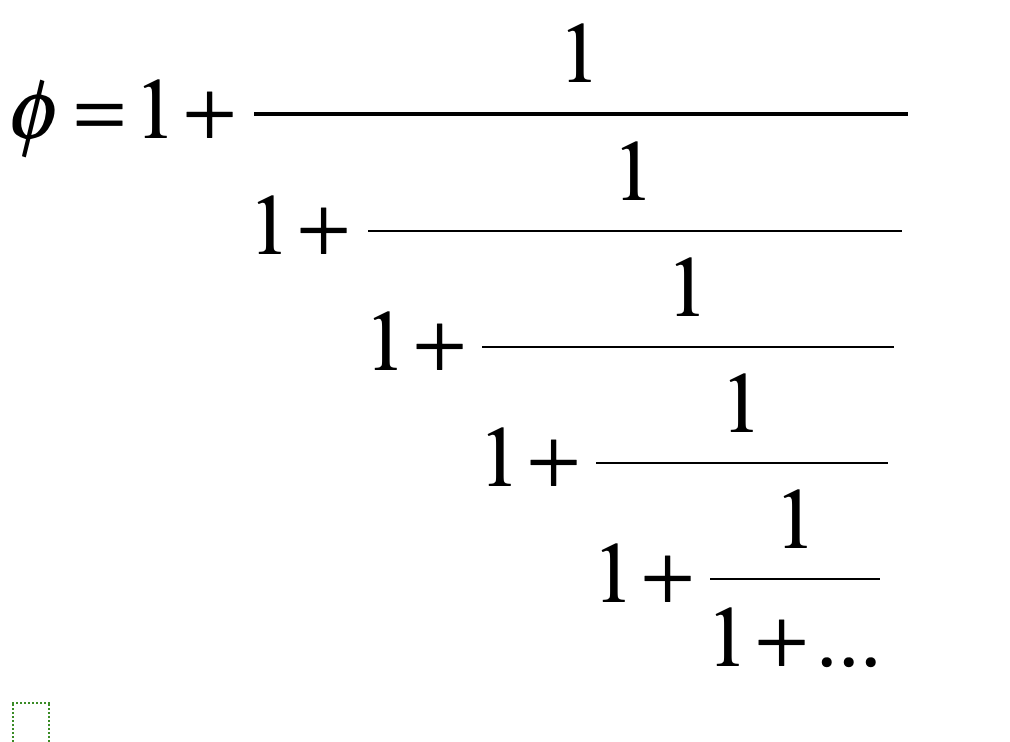
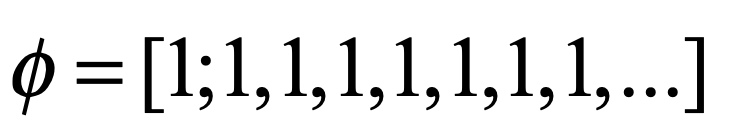


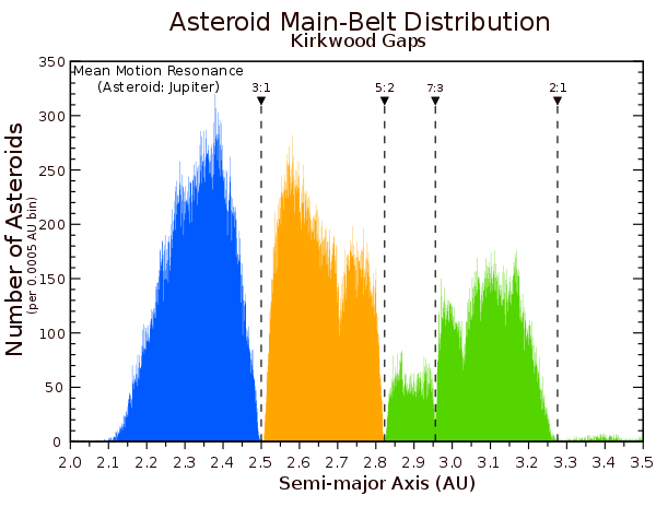

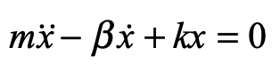
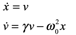
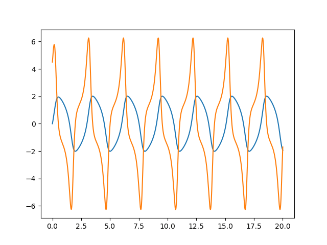
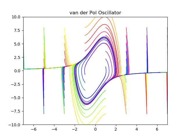
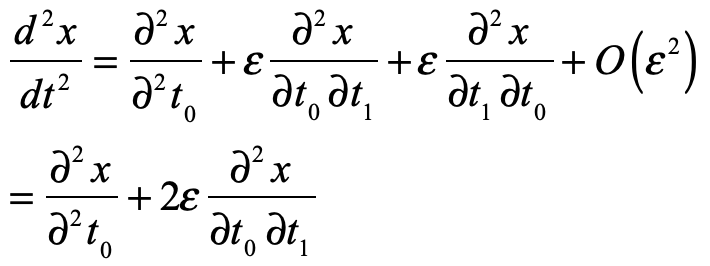
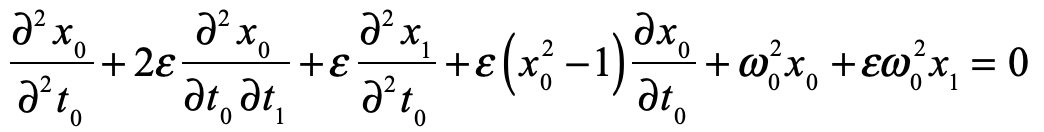
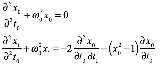
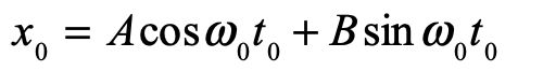
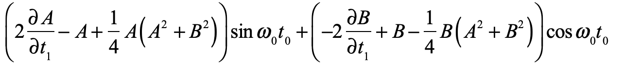
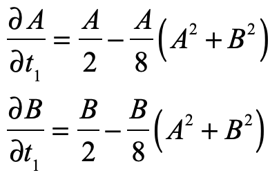
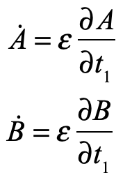
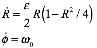
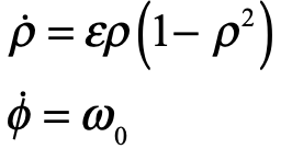
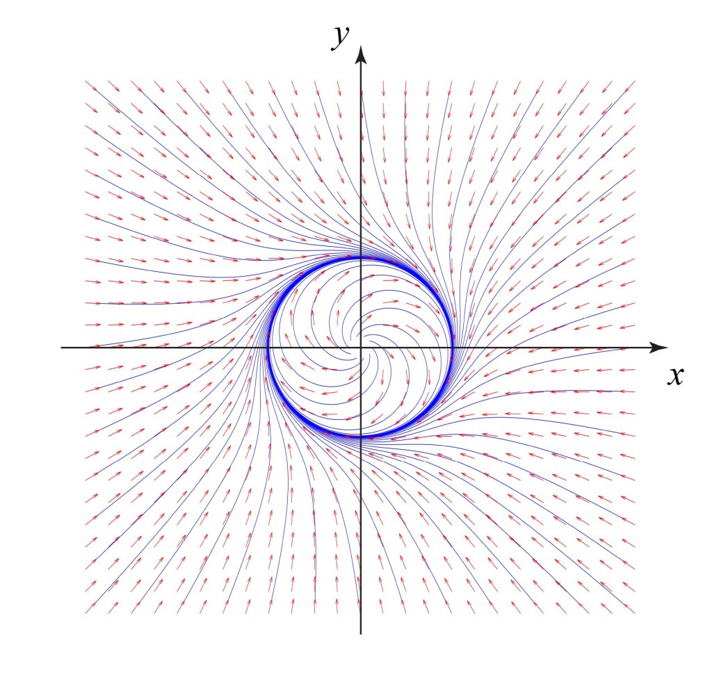


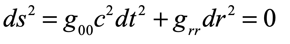


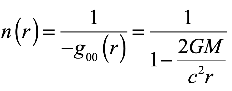
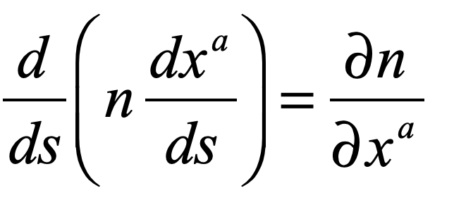
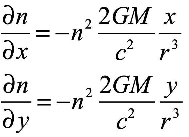


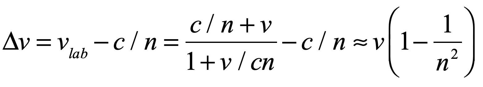


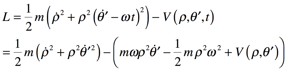
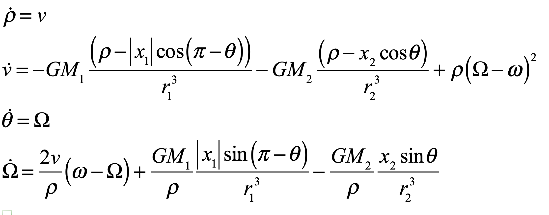
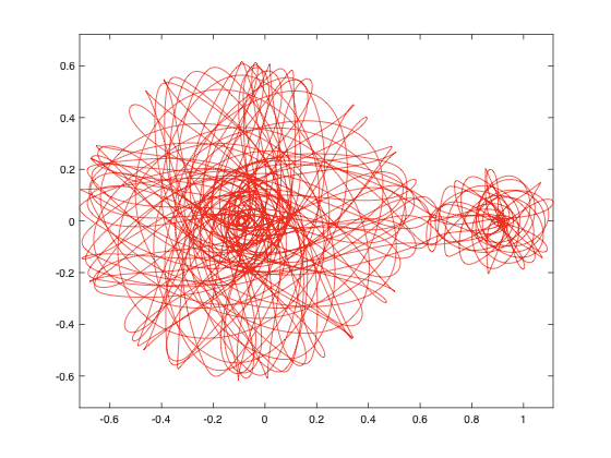

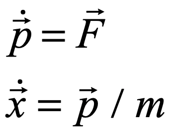
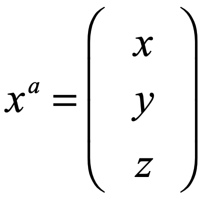
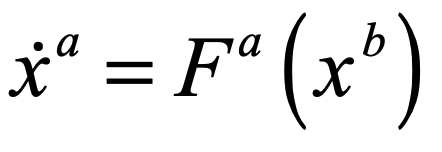
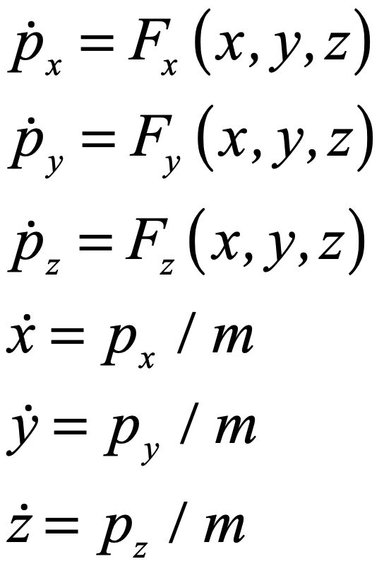
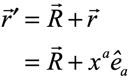
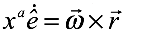
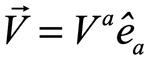
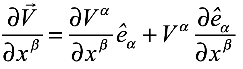
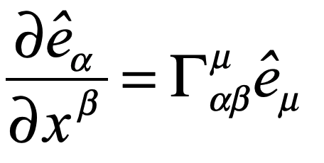
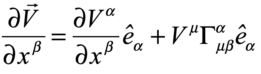
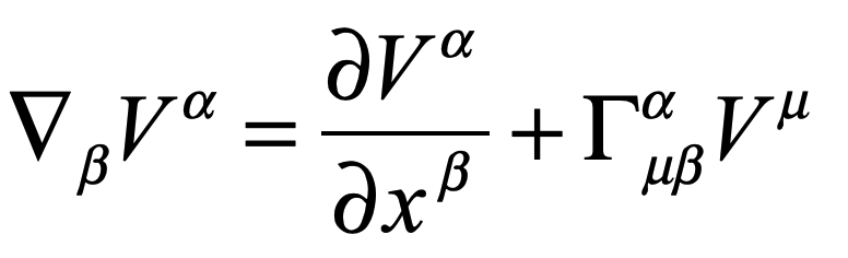
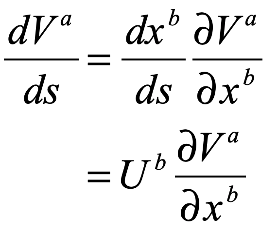
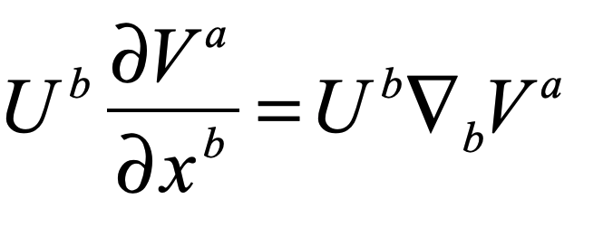
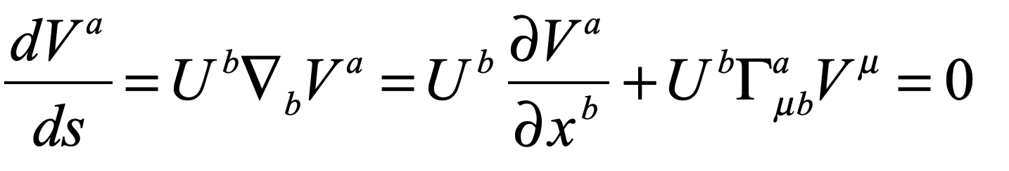
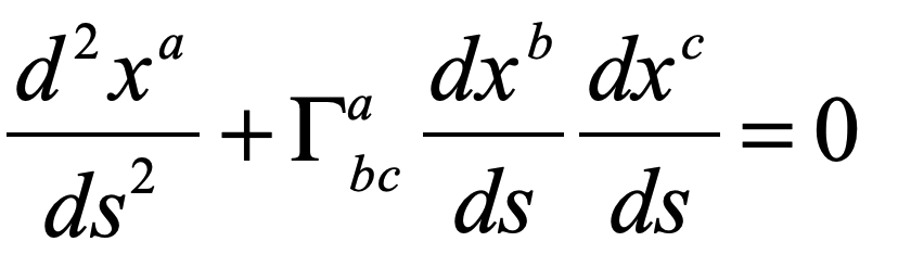

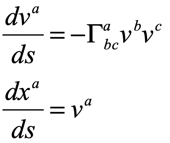
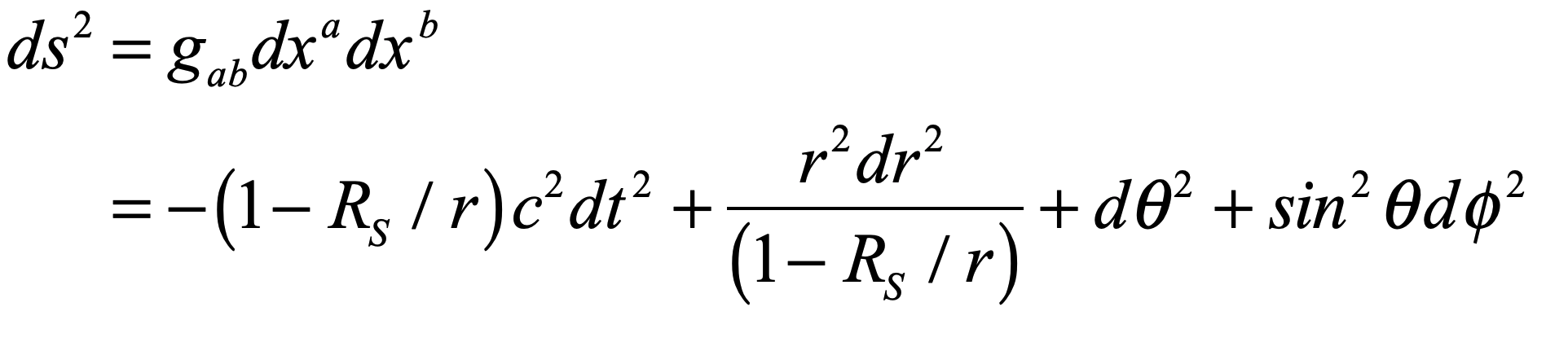
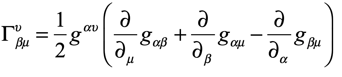

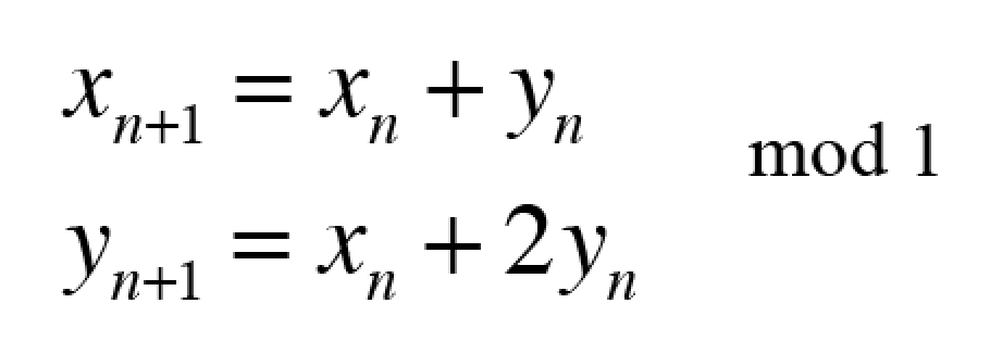
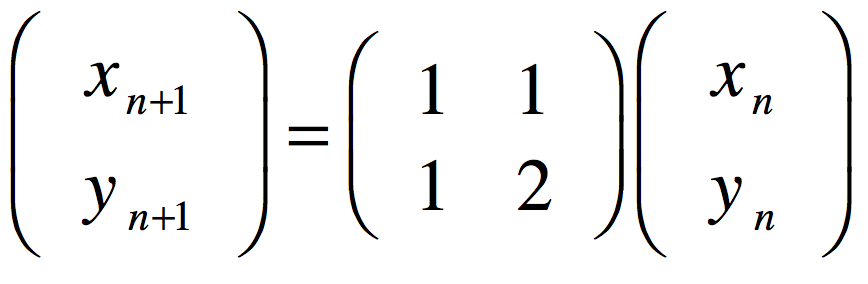


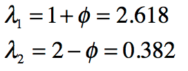
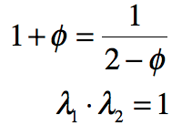
